Rice distribution

In the 2D plane, pick a fixed point at distance ν from the origin. Generate a distribution of 2D points centered around that point, where the x and y coordinates are chosen independently from a Gaussian distribution with standard deviation σ (blue region). If R is the distance from these points to the origin, then R has a Rice distribution.

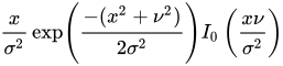
Probability density function
Cumulative distribution function
Notation	$\mathrm {Rice} (\nu ,\sigma )$
Parameters	$\nu \geq 0$, distance between the reference point and the center of the bivariate distribution, $\sigma \geq 0$, scale
Support	$x\in [0,\infty )$
PDF	${\frac {x}{\sigma ^{2}}}\exp \left({\frac {-(x^{2}+\nu ^{2})}{2\sigma ^{2}}}\right)I_{0}\left({\frac {x\nu }{\sigma ^{2}}}\right)$
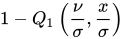
CDF	$1-Q_{1}\left({\frac {\nu }{\sigma }},{\frac {x}{\sigma }}\right)$ where Q1 is the Marcum Q-function
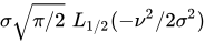
Mean	$\sigma {\sqrt {\pi /2}}\,\,L_{1/2}(-\nu ^{2}/2\sigma ^{2})$
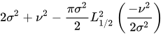
Variance	$2\sigma ^{2}+\nu ^{2}-{\frac {\pi \sigma ^{2}}{2}}L_{1/2}^{2}\left({\frac {-\nu ^{2}}{2\sigma ^{2}}}\right)$
Skewness	(complicated)
Excess kurtosis	(complicated)

In probability theory, the Rice distribution or Rician distribution (or, less commonly, Ricean distribution) is the probability distribution of the magnitude of a circularly symmetric bivariate normal random variable, possibly with non-zero mean (noncentral). It was named after Stephen O. Rice (1907–1986).

Characterization

The probability density function is

$f(x\mid \nu ,\sigma )={\frac {x}{\sigma ^{2}}}\exp \left({\frac {-(x^{2}+\nu ^{2})}{2\sigma ^{2}}}\right)I_{0}\left({\frac {x\nu }{\sigma ^{2}}}\right)H(x),$

where I₀(z) is the modified Bessel function of the first kind with order zero, and H(x) is the Heaviside unit step.

In the context of Rician fading, the distribution is often also rewritten using the shape parameter $K={\frac {\nu ^{2}}{2\sigma ^{2}}}$, defined as the ratio of the power contributions by line-of-sight path to the remaining multipaths, and the scale parameter $\Omega =\nu ^{2}+2\sigma ^{2}$, defined as the total power received in all paths.

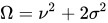
The characteristic function of the Rice distribution is given as:

${\begin{aligned}\chi _{X}(t\mid \nu ,\sigma )=\exp \left(-{\frac {\nu ^{2}}{2\sigma ^{2}}}\right)&\left[\Psi _{2}\left(1;1,{\frac {1}{2}};{\frac {\nu ^{2}}{2\sigma ^{2}}},-{\frac {1}{2}}\sigma ^{2}t^{2}\right)\right.\\[8pt]&\left.{}+i{\sqrt {2}}\sigma t\Psi _{2}\left({\frac {3}{2}};1,{\frac {3}{2}};{\frac {\nu ^{2}}{2\sigma ^{2}}},-{\frac {1}{2}}\sigma ^{2}t^{2}\right)\right],\end{aligned}}$

where ${\displaystyle \Psi _{2}\left(\alpha$ ;\gamma ,\gamma ';x,y\right)} is one of Horn's confluent hypergeometric functions with two variables and convergent for all finite values of $x$ and ⁠$y$⁠. It is given by:

${\displaystyle \Psi _{2}\left(\alpha$ ;\gamma ,\gamma ';x,y\right)=\sum _{n=0}^{\infty }\sum _{m=0}^{\infty }{\frac {(\alpha )_{m+n}}{(\gamma )_{m}(\gamma ')_{n}}}{\frac {x^{m}y^{n}}{m!n!}},}

where

$(x)_{n}=x(x+1)\cdots (x+n-1)={\frac {\Gamma (x+n)}{\Gamma (x)}}$

is the rising factorial.

Properties

Moments

The first few raw moments are:

${\begin{aligned}\mu _{1}^{'}&=\sigma {\sqrt {\pi /2}}\,\,L_{1/2}(-\nu ^{2}/2\sigma ^{2})\\\mu _{2}^{'}&=2\sigma ^{2}+\nu ^{2}\,\\\mu _{3}^{'}&=3\sigma ^{3}{\sqrt {\pi /2}}\,\,L_{3/2}(-\nu ^{2}/2\sigma ^{2})\\\mu _{4}^{'}&=8\sigma ^{4}+8\sigma ^{2}\nu ^{2}+\nu ^{4}\,\\\mu _{5}^{'}&=15\sigma ^{5}{\sqrt {\pi /2}}\,\,L_{5/2}(-\nu ^{2}/2\sigma ^{2})\\\mu _{6}^{'}&=48\sigma ^{6}+72\sigma ^{4}\nu ^{2}+18\sigma ^{2}\nu ^{4}+\nu ^{6}\end{aligned}}$

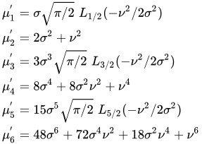
and, in general, the raw moments are given by

$\mu _{k}^{'}=\sigma ^{k}2^{k/2}\,\Gamma (1\!+\!k/2)\,L_{k/2}(-\nu ^{2}/2\sigma ^{2}).$

Here ⁠$L_{q}(x)$⁠ denotes a Laguerre polynomial:

$L_{q}(x)=L_{q}^{(0)}(x)=M(-q,1,x)=\,_{1}F_{1}(-q;1;x)$

where $M(a,b,z)=_{1}F_{1}(a;b;z)$ is the confluent hypergeometric function of the first kind. When ⁠$k$⁠ is even, the raw moments become simple polynomials in ⁠$\sigma$⁠ and ⁠$\nu$⁠, as in the examples above.

For the case ⁠$q=1/2$⁠:

${\begin{aligned}L_{1/2}(x)&=\,_{1}F_{1}\left(-{\frac {1}{2}};1;x\right)\\&=e^{x/2}\left[\left(1-x\right)I_{0}\left(-{\frac {x}{2}}\right)-xI_{1}\left(-{\frac {x}{2}}\right)\right].\end{aligned}}$

The second central moment, the variance, is

$\mu _{2}=2\sigma ^{2}+\nu ^{2}-(\pi \sigma ^{2}/2)\,L_{1/2}^{2}(-\nu ^{2}/2\sigma ^{2}).$

Note that $L_{1/2}^{2}(\cdot )$ indicates the square of the Laguerre polynomial ⁠$L_{1/2}(\cdot )$⁠, not the generalized Laguerre polynomial ⁠$L_{1/2}^{(2)}(\cdot )$⁠.

Related distributions

• $R\sim \mathrm {Rice} \left(|\nu |,\sigma \right)$ if $R={\sqrt {X^{2}+Y^{2}}}$ where $X\sim N\left(\nu \cos \theta ,\sigma ^{2}\right)$ and $Y\sim N\left(\nu \sin \theta ,\sigma ^{2}\right)$ are statistically independent normal random variables and $\theta$ is any real number.
• Another case where $R\sim \mathrm {Rice} \left(\nu ,\sigma \right)$ comes from the following steps:
  1. Generate $P$ having a Poisson distribution with parameter (also mean, for a Poisson) ⁠$\textstyle \lambda ={\frac {\nu ^{2}}{2\sigma ^{2}}}$⁠.
  2. Generate $X$ having a chi-squared distribution with ⁠$2P+2$⁠ degrees of freedom.
  3. Set $R=\sigma {\sqrt {X}}.$
• If $R\sim \operatorname {Rice} (\nu ,1)$ then $R^{2}$ has a noncentral chi-squared distribution with two degrees of freedom and noncentrality parameter ⁠$\nu ^{2}$⁠.
• If $R\sim \operatorname {Rice} (\nu ,1)$ then $R$ has a noncentral chi distribution with two degrees of freedom and noncentrality parameter ⁠$\nu$⁠.
• If $R\sim \operatorname {Rice} (0,\sigma )$ then ⁠$R\sim \operatorname {Rayleigh} (\sigma )$⁠, i.e., for the special case of the Rice distribution given by $\nu =0$, the distribution becomes the Rayleigh distribution, for which the variance is ⁠$\textstyle \mu _{2}={\frac {4-\pi }{2}}\sigma ^{2}$⁠.
• If $R\sim \operatorname {Rice} (0,\sigma )$ then $R^{2}$ has an exponential distribution.
• If $R\sim \operatorname {Rice} \left(\nu ,\sigma \right)$ then $1/R$ has an Inverse Rician distribution.
• The folded normal distribution is the univariate restriction of the Rice distribution.

Limiting cases

For large values of the argument, the Laguerre polynomial becomes

$\lim _{x\to -\infty }L_{\nu }(x)={\frac {|x|^{\nu }}{\Gamma (1+\nu )}}.$

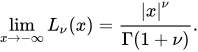
It is seen that as ⁠$\nu$⁠ becomes large or ⁠$\sigma$⁠ becomes small, the mean becomes ⁠$\nu$⁠ and the variance becomes ⁠$\sigma ^{2}$⁠.

The transition to a Gaussian approximation proceeds as follows. From Bessel function theory we have

$I_{\alpha }(z)\to {\frac {e^{z}}{\sqrt {2\pi z}}}\left(1-{\frac {4\alpha ^{2}-1}{8z}}+\cdots \right){\text{ as }}z\rightarrow \infty$

so, in the large $x\nu /\sigma ^{2}$ region, an asymptotic expansion of the Rician distribution:

${\begin{aligned}f(x,\nu ,\sigma )={}&{\frac {x}{\sigma ^{2}}}\exp \left({\frac {-(x^{2}+\nu ^{2})}{2\sigma ^{2}}}\right)I_{0}\left({\frac {x\nu }{\sigma ^{2}}}\right)\\{\text{ is }}\\&{\frac {x}{\sigma ^{2}}}\exp \left({\frac {-(x^{2}+\nu ^{2})}{2\sigma ^{2}}}\right){\sqrt {\frac {\sigma ^{2}}{2\pi x\nu }}}\exp \left({\frac {2x\nu }{2\sigma ^{2}}}\right)\left(1+{\frac {\sigma ^{2}}{8x\nu }}+\cdots \right)\\\rightarrow {}&{\frac {1}{\sigma {\sqrt {2\pi }}}}\exp \left(-{\frac {(x-\nu )^{2}}{2\sigma ^{2}}}\right){\sqrt {\frac {x}{\nu }}},\;\;\;{\text{ as }}{\frac {x\nu }{\sigma ^{2}}}\rightarrow \infty \end{aligned}}$

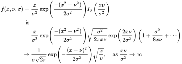
Moreover, when the density is concentrated around ${\textstyle \nu }$ and ${\textstyle |x-\nu |\ll \sigma }$ because of the Gaussian exponent, we can also write ${\textstyle {\sqrt {{x}/{\nu }}}\approx 1}$ and finally get the Normal approximation

$f(x,\nu ,\sigma )\approx {\frac {1}{\sigma {\sqrt {2\pi }}}}\exp \left(-{\frac {(x-\nu )^{2}}{2\sigma ^{2}}}\right),\;\;\;{\frac {\nu }{\sigma }}\gg 1$

The approximation becomes usable for ⁠${\nu }/{\sigma }>3$⁠.

Parameter estimation (Koay inversion technique)

There are three different methods for estimating the parameters of the Rice distribution, (1) method of moments, (2) method of maximum likelihood, and (3) method of least squares. In the first two methods the interest is in estimating the parameters of the distribution, ⁠$\nu$⁠ and ⁠$\sigma$⁠, from a sample of data. This can be done using the method of moments, e.g., the sample mean and the sample standard deviation. The sample mean is an estimate of ⁠$\mu _{1}^{'}$⁠ and the sample standard deviation is an estimate of ⁠$\mu _{2}^{1/2}$⁠.

The following is an efficient method, known as the "Koay inversion technique". for solving the estimating equations, based on the sample mean and the sample standard deviation, simultaneously . This inversion technique is also known as the fixed point formula of SNR. Earlier works on the method of moments usually use a root-finding method to solve the problem, which is not efficient.

First, the ratio of the sample mean to the sample standard deviation is defined as ⁠$r$⁠, i.e., ⁠$r=\mu _{1}^{'}/\mu _{2}^{1/2}$⁠. The fixed point formula of SNR is expressed as

$g(\theta )={\sqrt {\xi {(\theta )}\left[1+r^{2}\right]-2}},$

where $\theta$ is the ratio of the parameters, i.e., ⁠$\theta ={\nu }/{\sigma }$⁠, and $\xi {\left(\theta \right)}$ is given by:

$\xi {\left(\theta \right)}=2+\theta ^{2}-{\frac {\pi }{8}}\exp {(-\theta ^{2}/2)}\left[(2+\theta ^{2})I_{0}(\theta ^{2}/4)+\theta ^{2}I_{1}(\theta ^{2}/4)\right]^{2},$

where $I_{0}$ and $I_{1}$ are modified Bessel functions of the first kind.

Note that $\xi {\left(\theta \right)}$ is a scaling factor of $\sigma$ and is related to $\mu _{2}$ by:

$\mu _{2}=\xi {\left(\theta \right)}\sigma ^{2}.$

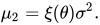
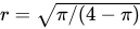
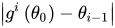
To find the fixed point, ⁠$\theta ^{*}$⁠, of ⁠$g$⁠, an initial solution is selected, ⁠${\theta }_{0}$⁠, that is greater than the lower bound, which is ${\theta }_{\text{lower bound}}=0$ and occurs when ${\textstyle r={\sqrt {\pi /(4-\pi )}}}$ (Notice that this is the $r=\mu _{1}^{'}/\mu _{2}^{1/2}$ of a Rayleigh distribution). This provides a starting point for the iteration, which uses functional composition, and this continues until $\left|g^{i}\left(\theta _{0}\right)-\theta _{i-1}\right|$ is less than some small positive value. Here, $g^{i}$ denotes the composition of the same function, ⁠$g$⁠, $i$ times. In practice, we associate the final $\theta _{n}$ for some integer $n$ as the fixed point, ⁠$\theta ^{*}$⁠, i.e., ⁠$\theta ^{*}=g\left(\theta ^{*}\right)$⁠.

Once the fixed point is found, the estimates $\nu$ and $\sigma$ are found through the scaling function, ⁠$\xi {\left(\theta \right)}$⁠, as follows:

$\sigma ={\frac {\mu _{2}^{1/2}}{\sqrt {\xi \left(\theta ^{*}\right)}}},$

and

$\nu ={\sqrt {\left(\mu _{1}^{'~2}+\left(\xi \left(\theta ^{*}\right)-2\right)\sigma ^{2}\right)}}.$

To speed up the iteration even more, one can use the Newton's method of root-finding. This particular approach is highly efficient.

Applications

• The Euclidean norm of a bivariate circularly symmetric normally distributed random vector.
• Rician fading (for multipath interference))
• Effect of sighting error on target shooting.
• Analysis of diversity receivers in radio communications.
• Distribution of eccentricities for models of the inner Solar System after long-term numerical integration.
• Distribution of noise in magnetic resonance imaging images is rician

See also

• Hoyt distribution
• Rayleigh distribution

Further reading

• Abramowitz, M. and Stegun, I. A. (ed.), Handbook of Mathematical Functions, National Bureau of Standards, 1964; reprinted Dover Publications, 1965. ISBN 0-486-61272-4
• Rice, S. O., Mathematical Analysis of Random Noise. Bell System Technical Journal 24 (1945) 46–156.
• I. Soltani Bozchalooi; Ming Liang (20 November 2007). "A smoothness index-guided approach to wavelet parameter selection in signal de-noising and fault detection". Journal of Sound and Vibration. 308 (1–2): 253–254. Bibcode:2007JSV...308..246B. doi:10.1016/j.jsv.2007.07.038.
• Wang, Dong; Zhou, Qiang; Tsui, Kwok-Leung (2017). "On the distribution of the modulus of Gabor wavelet coefficients and the upper bound of the dimensionless smoothness index in the case of additive Gaussian noises: Revisited". Journal of Sound and Vibration. 395: 393–400. doi:10.1016/j.jsv.2017.02.013.
• Liu, X. and Hanzo, L., A Unified Exact BER Performance Analysis of Asynchronous DS-CDMA Systems Using BPSK Modulation over Fading Channels, IEEE Transactions on Wireless Communications, Volume 6, Issue 10, October 2007, pp. 3504–3509.
• Annamalai, A., Tellambura, C. and Bhargava, V. K., Equal-Gain Diversity Receiver Performance in Wireless Channels, IEEE Transactions on Communications, Volume 48, October 2000, pp. 1732–1745.
• Erdelyi, A., Magnus, W., Oberhettinger, F. and Tricomi, F. G., Higher Transcendental Functions, Volume 1. Archived 11 August 2011 at the Wayback Machine McGraw-Hill Book Company Inc., 1953.
• Srivastava, H. M. and Karlsson, P. W., Multiple Gaussian Hypergeometric Series. Ellis Horwood Ltd., 1985.
• Sijbers J., den Dekker A. J., Scheunders P. and Van Dyck D., "Maximum Likelihood estimation of Rician distribution parameters" Archived 19 October 2011 at the Wayback Machine, IEEE Transactions on Medical Imaging, Vol. 17, Nr. 3, pp. 357–361, (1998)
• Varadarajan D. and Haldar J. P., "A Majorize-Minimize Framework for Rician and Non-Central Chi MR Images", IEEE Transactions on Medical Imaging, Vol. 34, no. 10, pp. 2191–2202, (2015)
• den Dekker, A.J.; Sijbers, J (December 2014). "Data distributions in magnetic resonance images: a review". Physica Medica. 30 (7): 725–741. doi:10.1016/j.ejmp.2014.05.002. PMID 25059432.
• Koay, C.G. and Basser, P. J., Analytically exact correction scheme for signal extraction from noisy magnitude MR signals, Journal of Magnetic Resonance, Volume 179, Issue = 2, pp. 317–322, (2006)
• Abdi, A., Tepedelenlioglu, C., Kaveh, M., and Giannakis, G. On the estimation of the K parameter for the Rice fading distribution, IEEE Communications Letters, Volume 5, Number 3, March 2001, pp. 92–94.
• Talukdar, K.K.; Lawing, William D. (March 1991). "Estimation of the parameters of the Rice distribution". Journal of the Acoustical Society of America. 89 (3): 1193–1197. Bibcode:1991ASAJ...89.1193T. doi:10.1121/1.400532.
• Bonny, J.M.; Renou, J.P.; Zanca, M. (November 1996). "Optimal Measurement of Magnitude and Phase from MR Data". Journal of Magnetic Resonance, Series B. 113 (2): 136–144. Bibcode:1996JMRB..113..136B. doi:10.1006/jmrb.1996.0166. PMID 8954899.

External links

• MATLAB code for Rice/Rician distribution (PDF, mean and variance, and generating random samples)