Noncentral t-distribution

Noncentral Student's t
Probability density function
Parameters	ν > 0 degrees of freedom $\mu \in \Re \,\!$ noncentrality parameter
Support	${\displaystyle x\in (-\infty$ ;+\infty )\,\!}
PDF	see text
CDF	see text
Mean	see text
Mode	see text
Variance	see text
Skewness	see text
Excess kurtosis	see text

The noncentral t-distribution generalizes Student's t-distribution using a noncentrality parameter. Whereas the central probability distribution describes how a test statistic t is distributed when the difference tested is null, the noncentral distribution describes how t is distributed when the null is false. This leads to its use in statistics, especially calculating statistical power. The noncentral t-distribution is also known as the singly noncentral t-distribution, and in addition to its primary use in statistical inference, is also used in robust modeling for data.

Definitions

If Z is a standard normal random variable, and V is a chi-squared distributed random variable with ν degrees of freedom that is independent of Z, then

$T={\frac {Z+\mu }{\sqrt {V/\nu }}}$

is a noncentral t-distributed random variable with ν degrees of freedom and noncentrality parameter μ ≠ 0. Note that the noncentrality parameter may be negative.

Cumulative distribution function

The cumulative distribution function of noncentral t-distribution with ν degrees of freedom and noncentrality parameter μ can be defined using the integral

$F_{\nu ,\mu }(x)={\frac {1}{2^{\nu /2-1}\Gamma (\nu /2)}}\int _{0}^{\infty }\Phi \left({\frac {ux}{\sqrt {\nu }}}-\mu \right)u^{\nu -1}e^{-{\frac {1}{2}}u^{2}}du,$

where $\Phi (x)$ is the cumulative distribution function of the standard normal distribution. A more practical approach is to express it as

$F_{\nu ,\mu }(x)={\begin{cases}{\tilde {F}}_{\nu ,\mu }(x),&{\mbox{if }}x\geq 0;\\1-{\tilde {F}}_{\nu ,-\mu }(x),&{\mbox{if }}x<0,\end{cases}}$

where

${\tilde {F}}_{\nu ,\mu }(x)=\Phi (-\mu )+{\frac {1}{2}}\sum _{j=0}^{\infty }\left[p_{j}I_{y}\left(j+{\frac {1}{2}},{\frac {\nu }{2}}\right)+q_{j}I_{y}\left(j+1,{\frac {\nu }{2}}\right)\right],$

$I_{y}\,\!(a,b)$ is the regularized incomplete beta function,

$y={\frac {x^{2}}{x^{2}+\nu }},$

$p_{j}={\frac {1}{j!}}\exp \left(-{\frac {\mu ^{2}}{2}}\right)\left({\frac {\mu ^{2}}{2}}\right)^{j},$

$q_{j}={\frac {\mu }{{\sqrt {2}}\Gamma (j+3/2)}}\exp \left(-{\frac {\mu ^{2}}{2}}\right)\left({\frac {\mu ^{2}}{2}}\right)^{j},$

Although this formula is more complicated, it is computationally more efficient, as each series term can be calculated from the previous term using simple arithmetic operations. In statistical programming language R, the cumulative distribution function is implemented as pt. In the Python library SciPy, it is implemented as scipy.stats.nct.cdf.

Probability density function

The probability density function (pdf) for the noncentral t-distribution with ν > 0 degrees of freedom and noncentrality parameter μ can be expressed in several forms. A simple integral form is given by:

$f(x)={\frac {2^{\frac {1-\nu }{2}}}{{\sqrt {\nu \pi }}\,\Gamma (\nu /2)}}\int _{0}^{\infty }u^{\nu }\exp \left(-{\frac {1}{2}}\left({\frac {ux}{\sqrt {\nu }}}-\mu \right)^{2}-{\frac {1}{2}}u^{2}\right)du$

The confluent hypergeometric function form of the density function is

$f(x)=\underbrace {{\frac {\Gamma ({\frac {\nu +1}{2}})}{{\sqrt {\nu \pi }}\,\Gamma ({\frac {\nu }{2}})}}\left(1+{\frac {x^{2}}{\nu }}\right)^{-{\tfrac {\nu +1}{2}}}} _{{\text{StudentT}}(x\,;\,\mu =0)}\exp \left(-{\frac {\mu ^{2}}{2}}\right){\Big (}A_{\nu }(x\,;\,\mu )+B_{\nu }(x\,;\,\mu ){\Big )},$

where

${\begin{aligned}A_{\nu }(x\,;\,\mu )&={_{1}F}_{1}\left({\frac {\nu +1}{2}}\,;\,{\frac {1}{2}}\,;\,{\frac {\mu ^{2}x^{2}}{2(x^{2}+\nu )}}\right),\\B_{\nu }(x\,;\,\mu )&={\frac {{\sqrt {2}}\mu x}{\sqrt {x^{2}+\nu }}}{\frac {\Gamma ({\frac {\nu }{2}}+1)}{\Gamma ({\frac {\nu +1}{2}})}}{_{1}F}_{1}\left({\frac {\nu }{2}}+1\,;\,{\frac {3}{2}}\,;\,{\frac {\mu ^{2}x^{2}}{2(x^{2}+\nu )}}\right),\end{aligned}}$

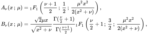
and where ₁F₁ is a confluent hypergeometric function.

An alternative integral form is

$f(x)={\frac {\nu ^{\frac {\nu }{2}}\exp \left(-{\frac {\nu \mu ^{2}}{2(x^{2}+\nu )}}\right)}{{\sqrt {\pi }}\Gamma ({\frac {\nu }{2}})2^{\frac {\nu -1}{2}}(x^{2}+\nu )^{\frac {\nu +1}{2}}}}\int _{0}^{\infty }y^{\nu }\exp \left(-{\frac {1}{2}}\left(y-{\frac {\mu x}{\sqrt {x^{2}+\nu }}}\right)^{2}\right)dy.$

A third form of the density is obtained using its cumulative distribution functions, as follows.

$f(x)={\begin{cases}{\frac {\nu }{x}}\left\{F_{\nu +2,\mu }\left(x{\sqrt {1+{\frac {2}{\nu }}}}\right)-F_{\nu ,\mu }(x)\right\},&{\mbox{if }}x\neq 0;\\{\frac {\Gamma ({\frac {\nu +1}{2}})}{{\sqrt {\pi \nu }}\Gamma ({\frac {\nu }{2}})}}\exp \left(-{\frac {\mu ^{2}}{2}}\right),&{\mbox{if }}x=0.\end{cases}}$

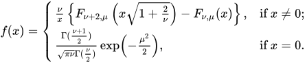
This is the approach implemented by the dt function in R.

Derivation

The integral form of the CDF can be derived directly from the definition of a noncentral t variable:

$F_{\nu ,\mu }(x)=\mathrm {P} \left\{{\frac {Z+\mu }{\sqrt {V/\nu }}}<x\right\}=\mathrm {P} \left\{{\frac {Z+\mu }{\chi /{\sqrt {\nu }}}}<x\right\},$

where $\chi$ represents a chi random variable with $\nu$ degrees of freedom. Since $Z$ and $\chi$ are independent random variables, the above probability can be quantified as the double integral of the product of their probability density functions over the region where the inequality holds:

$\mathrm {P} \left\{{\frac {Z+\mu }{\chi /{\sqrt {\nu }}}}<x\right\}=\iint _{R}f_{Z}(z)f_{\chi }(u)dzdu=\iint _{R}\left({\frac {1}{\sqrt {2\pi }}}e^{-{\frac {1}{2}}z^{2}}\right)\left({\frac {1}{2^{\nu /2-1}\Gamma (\nu /2)}}u^{\nu -1}e^{-{\frac {1}{2}}u^{2}}\right)dzdu,$

$\mathrm {where\ } R=\left\{(u,z)\left|\,u>0,\,{\frac {z+\mu }{u/{\sqrt {\nu }}}}<x\right.\right\}=\left\{(u,z)\left|\,u>0,\,z<{\frac {x}{\sqrt {\nu }}}u-\mu \right.\right\}$

Here, region $R$ represents the area in the $(u,z)$-plane lying to the right of the line $u=0$, and below the line $z={\frac {x}{\sqrt {\nu }}}u-\mu$. Thus, the integral can be written with specified limits:

$F_{\nu ,\mu }(x)=\int _{0}^{\infty }\int _{-\infty }^{{\frac {x}{\sqrt {\nu }}}u-\mu }\left({\frac {1}{\sqrt {2\pi }}}e^{-{\frac {1}{2}}z^{2}}\right)dz\left({\frac {1}{2^{\nu /2-1}\Gamma (\nu /2)}}u^{\nu -1}e^{-{\frac {1}{2}}u^{2}}\right)du$

Finally, integrating with respect to $z$ and separating the constant term yields:

$F_{\nu ,\mu }(x)={\frac {1}{2^{\nu /2-1}\Gamma (\nu /2)}}\int _{0}^{\infty }\Phi \left({\frac {ux}{\sqrt {\nu }}}-\mu \right)u^{\nu -1}e^{-{\frac {1}{2}}u^{2}}du$.

The formula for the PDF can be found by differentiating the CDF with respect to $x$:

$f(x)={\frac {d}{dx}}F_{\nu ,\mu }(x)={\frac {1}{2^{\nu /2-1}\Gamma (\nu /2)}}\int _{0}^{\infty }{\frac {d}{dx}}\left[\Phi \left({\frac {ux}{\sqrt {\nu }}}-\mu \right)\right]u^{\nu -1}e^{-{\frac {1}{2}}u^{2}}du$

This simplifies to the first integral form of the PDF given above:

$f(x)={\frac {2^{\frac {1-\nu }{2}}}{{\sqrt {\nu \pi }}\,\Gamma (\nu /2)}}\int _{0}^{\infty }u^{\nu }\exp \left(-{\frac {1}{2}}\left({\frac {ux}{\sqrt {\nu }}}-\mu \right)^{2}-{\frac {1}{2}}u^{2}\right)du$

Properties

Moments of the noncentral t-distribution

In general, the kth raw moment of the noncentral t-distribution is

${\mbox{E}}\left[T^{k}\right]={\begin{cases}\left({\frac {\nu }{2}}\right)^{\frac {k}{2}}{\frac {\Gamma \left({\frac {\nu -k}{2}}\right)}{\Gamma \left({\frac {\nu }{2}}\right)}}{\mbox{exp}}\left(-{\frac {\mu ^{2}}{2}}\right){\frac {d^{k}}{d\mu ^{k}}}{\mbox{exp}}\left({\frac {\mu ^{2}}{2}}\right),&{\mbox{if }}\nu >k;\\{\mbox{Does not exist}},&{\mbox{if }}\nu \leq k.\\\end{cases}}$

In particular, the mean and variance of the noncentral t-distribution are

${\begin{aligned}{\mbox{E}}\left[T\right]&={\begin{cases}\mu {\sqrt {\frac {\nu }{2}}}{\frac {\Gamma ((\nu -1)/2)}{\Gamma (\nu /2)}},&{\mbox{if }}\nu >1;\\{\mbox{Does not exist}},&{\mbox{if }}\nu \leq 1,\\\end{cases}}\\{\mbox{Var}}\left[T\right]&={\begin{cases}{\frac {\nu (1+\mu ^{2})}{\nu -2}}-{\frac {\mu ^{2}\nu }{2}}\left({\frac {\Gamma ((\nu -1)/2)}{\Gamma (\nu /2)}}\right)^{2},&{\mbox{if }}\nu >2;\\{\mbox{Does not exist}},&{\mbox{if }}\nu \leq 2.\\\end{cases}}\end{aligned}}$

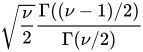
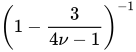
An excellent approximation to ${\sqrt {\frac {\nu }{2}}}{\frac {\Gamma ((\nu -1)/2)}{\Gamma (\nu /2)}}$ is $\left(1-{\frac {3}{4\nu -1}}\right)^{-1}$, which can be used in both formulas.

Asymmetry

The non-central t-distribution is asymmetric unless μ is zero, i.e., a central t-distribution. In addition, the asymmetry becomes smaller the larger degree of freedom. The right tail will be heavier than the left when μ > 0, and vice versa. However, the usual skewness is not generally a good measure of asymmetry for this distribution, because if the degrees of freedom is not larger than 3, the third moment does not exist at all. Even if the degrees of freedom is greater than 3, the sample estimate of the skewness is still very unstable unless the sample size is very large.

Mode

The noncentral t-distribution is always unimodal and bell shaped, but the mode is not analytically available, although for μ ≠ 0 we have

${\sqrt {\frac {\nu }{\nu +(5/2)}}}<{\frac {\mathrm {mode} }{\mu }}<{\sqrt {\frac {\nu }{\nu +1}}}$

In particular, the mode always has the same sign as the noncentrality parameter μ. Moreover, the negative of the mode is exactly the mode for a noncentral t-distribution with the same number of degrees of freedom ν but noncentrality parameter −μ.

The mode is strictly increasing with μ (it always moves in the same direction as μ is adjusted in). In the limit, when μ → 0, the mode is approximated by

${\displaystyle {\sqrt {\frac {\nu }{2}}}{\frac {\Gamma \left({\frac {\nu +2}{2}}\right)}{\Gamma \left({\frac {\nu +3}{2}}\right)}}\mu$ ;\,}

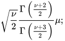
and when μ → ∞, the mode is approximated by

${\sqrt {\frac {\nu }{\nu +1}}}\mu .$

Related distributions

• Central t-distribution: the central t-distribution can be converted into a location/scale family. This family of distributions is used in data modeling to capture various tail behaviors. The location/scale generalization of the central t-distribution is a different distribution from the noncentral t-distribution discussed in this article. In particular, this approximation does not respect the asymmetry of the noncentral t-distribution. However, the central t-distribution can be used as an approximation to the noncentral t-distribution.
• If T is noncentral t-distributed with ν degrees of freedom and noncentrality parameter μ and F = T², then F has a noncentral F-distribution with 1 numerator degree of freedom, ν denominator degrees of freedom, and noncentrality parameter μ².
• If T is noncentral t-distributed with ν degrees of freedom and noncentrality parameter μ and $Z=\lim _{\nu \rightarrow \infty }T$, then Z has a normal distribution with mean μ and unit variance.
• When the denominator noncentrality parameter of a doubly noncentral t-distribution is zero, then it becomes a noncentral t-distribution.

Special cases

• When μ = 0, the noncentral t-distribution becomes the central (Student's) t-distribution with the same degrees of freedom.

Occurrence and applications

Use in power analysis

Suppose we have an independent and identically distributed sample X₁, ..., X_n each of which is normally distributed with mean θ and variance σ², and we are interested in testing the null hypothesis θ = 0 vs. the alternative hypothesis θ ≠ 0. We can perform a one sample t-test using the test statistic

$T={\frac {\bar {X}}{{\hat {\sigma }}/{\sqrt {n}}}}={\frac {{\frac {{\bar {X}}-\theta }{(\sigma /{\sqrt {n}})}}+{\frac {\theta }{(\sigma /{\sqrt {n}})}}}{\sqrt {\left.\left({\frac {{\hat {\sigma }}^{2}}{\sigma ^{2}/(n-1)}}\right)\right/(n-1)}}}$

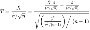
where ${\bar {X}}$ is the sample mean and ${\hat {\sigma }}^{2}\,\!$ is the unbiased sample variance. Since the right hand side of the second equality exactly matches the characterization of a noncentral t-distribution as described above, T has a noncentral t-distribution with n−1 degrees of freedom and noncentrality parameter ${\sqrt {n}}\theta /\sigma \,\!$.

If the test procedure rejects the null hypothesis whenever $|T|>t_{1-\alpha /2}\,\!$, where $t_{1-\alpha /2}\,\!$ is the upper α/2 quantile of the (central) Student's t-distribution for a pre-specified α ∈ (0, 1), then the power of this test is given by

$1-F_{n-1,{\sqrt {n}}\theta /\sigma }(t_{1-\alpha /2})+F_{n-1,{\sqrt {n}}\theta /\sigma }(-t_{1-\alpha /2}).$

Similar applications of the noncentral t-distribution can be found in the power analysis of the general normal-theory linear models, which includes the above one sample t-test as a special case.

Use in tolerance intervals

One-sided normal tolerance intervals have an exact solution in terms of the sample mean and sample variance based on the noncentral t-distribution. This enables the calculation of a statistical tolerance limit below which, with some confidence level, a specified proportion of a sampled population falls.

Let $X$ be a random normal variable with unknown population mean and variance, and let a sample of size $n$ yield sample mean ${\overline {x}}$ and sample standard deviation $s$. The probability that the proportion of $X$ values lying below limit $L$ is at least $p$ is given by the noncentral t-CDF:

$\mathrm {P} \left\{\mathrm {P} \left\{X<L\right\}>p\right\}=F_{\nu ,\mu }\left({\frac {L-{\overline {x}}}{s/{\sqrt {n}}}}\right),\ \ \mathrm {where\ } \nu =n-1,\ \ \mu =\Phi ^{-1}(p){\sqrt {n}}$

Tolerance bounds are typically expressed in the form ${\overline {x}}+ks$, where k is referred to as its k-factor. This factor is analogous to a z-score, but uses sample statistics rather than population parameters. In this framing, the probability that the proportion of $X$ lying below the limit ${\overline {x}}+ks$ is at least $p$ is given by

$\mathrm {P} \left\{\mathrm {P} \left\{X<{\overline {x}}+ks\right\}>p\right\}=F_{\nu ,\mu }({\sqrt {n}}k),\ \ \mathrm {where\ } \nu =n-1,\ \ \mu =\Phi ^{-1}(p){\sqrt {n}}$

Thus, calculating the k-factor corresponding to a given proportion and confidence level requires using the inverse cumulative distribution function of the noncentral t-distribution, which is implemented as qt in R, and as scipy.stats.nct.ppf in SciPy.

See also

• Noncentral F-distribution

External links

• Eric W. Weisstein. "Noncentral Student's t-Distribution." From MathWorld—A Wolfram Web Resource
• High accuracy calculation for life or science.: Noncentral t-distribution From Casio company.