Linear Regression using Boston Housing Dataset

Linear Regression predicts a continuous target value by finding the relationship between input features and the target variable. The Boston Housing dataset contains 506 instances and 13 features related to housing and neighborhood characteristics. The target variable represents the median value of owner-occupied homes. It includes:

• CRIM: Per capita crime rate by town.
• ZN: Proportion of residential land zoned for large lots.
• INDUS: Proportion of non-retail business acres per town.
• CHAS: Charles River dummy variable.
• NOX: Nitric oxide concentration.
• RM: Average number of rooms per dwelling.
• AGE: Proportion of owner-occupied units built before 1940.
• DIS: Weighted distance to employment centers.
• RAD: Index of accessibility to radial highways.
• TAX: Property-tax rate.
• PTRATIO: Pupil-teacher ratio by town.
• B: Proportion of the population by the given transformation of the Black population variable.
• LSTAT: Percentage of lower-status population.

Note: The original Boston Housing dataset has been removed from recent versions of scikit-learn. The example uses the OpenML version of the dataset for demonstration.

Implementation of Linear Regression

Step 1: Import Libraries and Dataset

First, import the required libraries and load the Boston Housing dataset from OpenML.

import numpy as np
import pandas as pd
import matplotlib.pyplot as plt

from sklearn.datasets import fetch_openml

boston = fetch_openml(name="boston", version=1, as_frame=True)

Explanation:

• NumPy: Provides support for numerical operations.
• Pandas: Handles the dataset using DataFrames.
• Matplotlib: Creates plots for visualizing model results.
• fetch_openml: Loads the Boston Housing dataset from OpenML.
• as_frame=True: Loads the feature data as a pandas DataFrame.

Step 2: Exploring the Dataset

Before preparing the data, check the dimensions of the feature dataset and view the available feature names.

boston.data.shape

Output:

Explanation:

• shape: Returns the number of rows and columns in the feature dataset.
• The Boston Housing dataset contains 506 rows and 13 features.

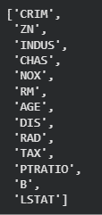
To view the names of all input features:

boston.feature_names

Output:

The output contains the 13 feature names:

Explanation:

• eature_names: Returns the names of the input features.
• These features describe different housing and neighborhood characteristics.

Step 3: Creating the DataFrame

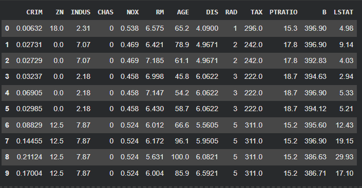
The feature data is converted into a pandas DataFrame, and the feature names are assigned as column names.

data = pd.DataFrame(boston.data)
data.columns = boston.feature_names

data.head(10)

Output:

Explanation:

• pd.DataFrame(boston.data): Creates a DataFrame from the feature data.
• data.columns: Assigns the 13 feature names as column headers.
• head(10): Displays the first 10 rows of the dataset.

Step 4: Adding the Target Variable

The target variable contains the house prices that the Linear Regression model will learn to predict. We first check the shape of the target data and then add it to the DataFrame as the Price column.

boston.target.shape

Output:

Explanation:

• boston.target: Contains the target values for all 506 records.
• shape: Returns the number of target values in the dataset.
• The target contains one value for each row in the feature dataset.

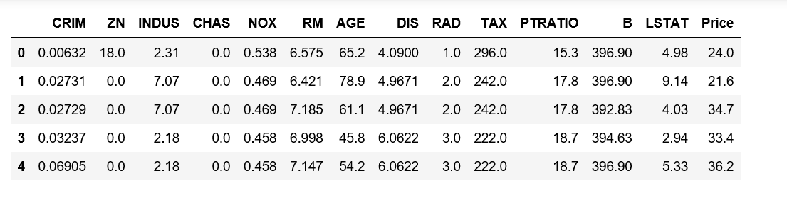
Add the target column:

data['Price'] = boston.target
data.head()

Output:

Explanation:

• data['Price']: Creates a new column named Price.
• boston.target: Provides the corresponding target value for each record.
• head(): Displays the first five rows after adding the target column.
• The DataFrame now contains the 13 input features and the target variable.

Step 5: Understanding the Dataset

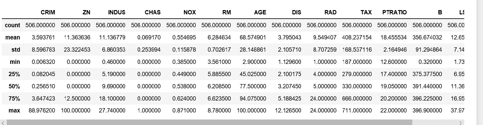
Before training the model, we can inspect the statistical summary of the numerical features.

data.describe()

Output:

Explanation:

• describe(): Generates statistical information for numerical columns.
• It shows values such as count, mean, standard deviation, minimum, maximum, and quartiles.
• This helps understand the distribution and range of the dataset features.

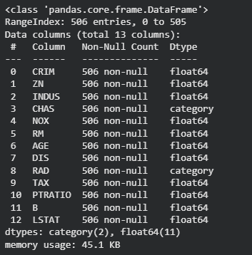
We can also check the structure and data types:

data.info()

Output:

Explanation:

• info(): Displays the number of rows, columns, data types, and non-null values.
• It helps verify the structure of the dataset.
• It can also be used to identify missing values.

Step 6: Preparing Training and Testing Data

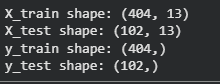
The dataset is divided into input features and target values. The input features are stored in X, while the house prices are stored in y.

X = boston.data
y = boston.target

from sklearn.model_selection import train_test_split

X_train, X_test, y_train, y_test = train_test_split(
    X,
    y,
    test_size=0.2,
    random_state=0
)

print("X_train shape:", X_train.shape)
print("X_test shape:", X_test.shape)
print("y_train shape:", y_train.shape)
print("y_test shape:", y_test.shape)

Output:

Explanation:

• X: Contains the 13 input features used for prediction.
• y: Contains the target house prices.
• train_test_split(): Divides the dataset into training and testing sets.
• test_size=0.2: Uses 20% of the data for testing and 80% for training.
• random_state=0: Ensures the same data split each time the code runs.
• X_train and y_train: Used to train the model.
• X_test and y_test: Used to evaluate the model.
• The training set contains 404 records, while the testing set contains 102 records.

Step 7: Training the Linear Regression Model

After splitting the dataset, we create a Linear Regression model and train it using the training data.

from sklearn.linear_model import LinearRegression

regressor = LinearRegression()
regressor.fit(X_train, y_train)

Output:

Explanation:

• LinearRegression: Provides the Linear Regression algorithm from scikit-learn.
• regressor: Stores the Linear Regression model.
• fit(): Trains the model using the input features and their corresponding target values.
• The model learns the relationship between the housing features and house prices.
• Plotting Scatter graph to show the prediction results - 'y_true' value vs 'y_pred' value.

Step 8: Predicting House Prices

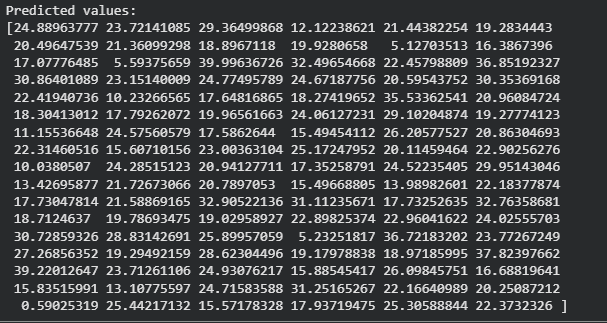
The trained model can now predict house prices for the test dataset.

y_pred = regressor.predict(X_test)

Output:

Explanation:

• predict(): Generates predictions using the trained model.
• X_test: Contains the housing features that were not used during training.
• y_pred: Stores the predicted house prices.
• The predicted values can be compared with y_test, which contains the actual house prices.

Step 9: Visualizing the Predictions

A scatter plot can be used to compare the actual house prices with the values predicted by the model.

plt.scatter(y_test, y_pred, c='green')
plt.xlabel("Price: in $1000's")
plt.ylabel("Predicted value")
plt.title("True Value vs Predicted Value: Linear Regression")
plt.show()

Output:

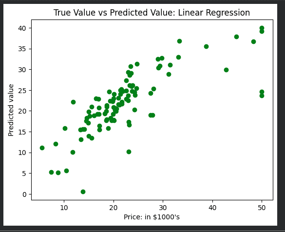
Explanation:

• plt.scatter(): Creates a scatter plot using actual and predicted values.
• y_test: Represents the actual house prices.
• y_pred: Represents the prices predicted by the model.
• xlabel(): Labels the horizontal axis with the actual prices.
• ylabel(): Labels the vertical axis with the predicted prices.
• Points closer to a diagonal pattern indicate that the predictions are closer to the actual values.
• Results of Linear Regression i.e. Mean Squared Error and Mean Absolute Error. 

Step 10: Evaluating the Model

We can evaluate the Linear Regression model using Mean Squared Error (MSE) and Mean Absolute Error (MAE).

from sklearn.metrics import mean_squared_error, mean_absolute_error
mse = mean_squared_error(ytest, y_pred)
mae = mean_absolute_error(ytest,y_pred)
print("Mean Square Error : ", mse)
print("Mean Absolute Error : ", mae)

Output:

Explanation:

• mean_squared_error(): Calculates the average squared difference between actual and predicted values.
• mean_absolute_error(): Calculates the average absolute difference between actual and predicted values.
• MSE: Penalizes larger prediction errors more heavily because the errors are squared.
• MAE: Represents the average absolute prediction error in the same unit as the target variable.
• Lower MSE and MAE values indicate better prediction performance.