3.7. softmax回归的简洁实现

Colab [mxnet]

Open the notebook in Colab

Colab [pytorch]

Open the notebook in Colab

Colab [tensorflow]

Open the notebook in Colab

Colab [paddle]

Open the notebook in Colab

SageMaker Studio Lab

Open the notebook in SageMaker Studio Lab

在 3.3节中， 我们发现通过深度学习框架的高级API能够使实现

线性回归变得更加容易。 同样，通过深度学习框架的高级API也能更方便地实现softmax回归模型。 本节如在 3.6节中一样， 继续使用Fashion-MNIST数据集，并保持批量大小为256。

mxnetpytorchtensorflowpaddle

from mxnet import gluon, init, npx
from mxnet.gluon import nn
from d2l import mxnet as d2l

npx.set_np()

batch_size = 256
train_iter, test_iter = d2l.load_data_fashion_mnist(batch_size)

[07:03:36] ../src/storage/storage.cc:196: Using Pooled (Naive) StorageManager for CPU

import torch
from torch import nn
from d2l import torch as d2l

batch_size = 256
train_iter, test_iter = d2l.load_data_fashion_mnist(batch_size)

import tensorflow as tf
from d2l import tensorflow as d2l

batch_size = 256
train_iter, test_iter = d2l.load_data_fashion_mnist(batch_size)

import warnings
from d2l import paddle as d2l

warnings.filterwarnings("ignore")
import paddle
from paddle import nn

batch_size = 256
train_iter, test_iter = d2l.load_data_fashion_mnist(batch_size)

Cache file /home/ci/.cache/paddle/dataset/fashion-mnist/train-images-idx3-ubyte.gz not found, downloading https://dataset.bj.bcebos.com/fashion_mnist/train-images-idx3-ubyte.gz
Begin to download
item 6451/6451 [============================>.] - ETA: 0s - 3ms/item
Download finished
Cache file /home/ci/.cache/paddle/dataset/fashion-mnist/train-labels-idx1-ubyte.gz not found, downloading https://dataset.bj.bcebos.com/fashion_mnist/train-labels-idx1-ubyte.gz
Begin to download
item 8/8 [============================>.] - ETA: 0s - 53ms/item
Download finished
Cache file /home/ci/.cache/paddle/dataset/fashion-mnist/t10k-images-idx3-ubyte.gz not found, downloading https://dataset.bj.bcebos.com/fashion_mnist/t10k-images-idx3-ubyte.gz
Begin to download
item 1080/1080 [============================>.] - ETA: 0s - 12ms/item
Download finished
Cache file /home/ci/.cache/paddle/dataset/fashion-mnist/t10k-labels-idx1-ubyte.gz not found, downloading https://dataset.bj.bcebos.com/fashion_mnist/t10k-labels-idx1-ubyte.gz
Begin to download
item 2/2 [=========================>....] - ETA: 0s - 2ms/item
Download finished

3.7.1. 初始化模型参数

如我们在 3.4节所述， softmax回归的输出层是一个全连接层。 因此，为了实现我们的模型， 我们只需在Sequential中添加一个带有10个输出的全连接层。 同样，在这里Sequential并不是必要的， 但它是实现深度模型的基础。 我们仍然以均值0和标准差0.01随机初始化权重。

mxnetpytorchtensorflowpaddle

net = nn.Sequential()
net.add(nn.Dense(10))
net.initialize(init.Normal(sigma=0.01))

# PyTorch不会隐式地调整输入的形状。因此，
# 我们在线性层前定义了展平层（flatten），来调整网络输入的形状
net = nn.Sequential(nn.Flatten(), nn.Linear(784, 10))

def init_weights(m):
    if type(m) == nn.Linear:
        nn.init.normal_(m.weight, std=0.01)

net.apply(init_weights);

net = tf.keras.models.Sequential()
net.add(tf.keras.layers.Flatten(input_shape=(28, 28)))
weight_initializer = tf.keras.initializers.RandomNormal(mean=0.0, stddev=0.01)
net.add(tf.keras.layers.Dense(10, kernel_initializer=weight_initializer))

net = nn.Sequential(nn.Flatten(), nn.Linear(784, 10))

def init_weights(m):
    if type(m) == nn.Linear:
        nn.initializer.Normal(m.weight, std=0.01)

net.apply(init_weights);

3.7.2. 重新审视Softmax的实现

在前面 3.6节的例子中， 我们计算了模型的输出，然后将此输出送入交叉熵损失。 从数学上讲，这是一件完全合理的事情。 然而，从计算角度来看，指数可能会造成数值稳定性问题。

回想一下，softmax函数\(\hat y_j = \frac{\exp(o_j)}{\sum_k \exp(o_k)}\)， 其中\(\hat y_j\)是预测的概率分布。 \(o_j\)是未规范化的预测\(\mathbf{o}\)的第\(j\)个元素。 如果\(o_k\)中的一些数值非常大， 那么\(\exp(o_k)\)可能大于数据类型容许的最大数字，即上溢（overflow）。 这将使分母或分子变为inf（无穷大）， 最后得到的是0、inf或nan（不是数字）的\(\hat y_j\)。 在这些情况下，我们无法得到一个明确定义的交叉熵值。

解决这个问题的一个技巧是： 在继续softmax计算之前，先从所有\(o_k\)中减去\(\max(o_k)\)。 这里可以看到每个\(o_k\)按常数进行的移动不会改变softmax的返回值：

(3.7.1)\[\begin{split}\begin{aligned} \hat y_j & = \frac{\exp(o_j - \max(o_k))\exp(\max(o_k))}{\sum_k \exp(o_k - \max(o_k))\exp(\max(o_k))} \\ & = \frac{\exp(o_j - \max(o_k))}{\sum_k \exp(o_k - \max(o_k))}. \end{aligned}\end{split}\]

在减法和规范化步骤之后，可能有些\(o_j - \max(o_k)\)具有较大的负值。 由于精度受限，\(\exp(o_j - \max(o_k))\)将有接近零的值，即下溢（underflow）。 这些值可能会四舍五入为零，使\(\hat y_j\)为零， 并且使得\(\log(\hat y_j)\)的值为-inf。 反向传播几步后，我们可能会发现自己面对一屏幕可怕的nan结果。

尽管我们要计算指数函数，但我们最终在计算交叉熵损失时会取它们的对数。 通过将softmax和交叉熵结合在一起，可以避免反向传播过程中可能会困扰我们的数值稳定性问题。 如下面的等式所示，我们避免计算\(\exp(o_j - \max(o_k))\)， 而可以直接使用\(o_j - \max(o_k)\)，因为\(\log(\exp(\cdot))\)被抵消了。

(3.7.2)\[\begin{split}\begin{aligned} \log{(\hat y_j)} & = \log\left( \frac{\exp(o_j - \max(o_k))}{\sum_k \exp(o_k - \max(o_k))}\right) \\ & = \log{(\exp(o_j - \max(o_k)))}-\log{\left( \sum_k \exp(o_k - \max(o_k)) \right)} \\ & = o_j - \max(o_k) -\log{\left( \sum_k \exp(o_k - \max(o_k)) \right)}. \end{aligned}\end{split}\]

我们也希望保留传统的softmax函数，以备我们需要评估通过模型输出的概率。 但是，我们没有将softmax概率传递到损失函数中， 而是在交叉熵损失函数中传递未规范化的预测，并同时计算softmax及其对数， 这是一种类似“LogSumExp技巧”的聪明方式。

mxnetpytorchtensorflowpaddle

loss = gluon.loss.SoftmaxCrossEntropyLoss()

loss = nn.CrossEntropyLoss(reduction='none')

loss = tf.keras.losses.SparseCategoricalCrossentropy(from_logits=True)

loss = nn.CrossEntropyLoss(reduction='none')

3.7.3. 优化算法

在这里，我们使用学习率为0.1的小批量随机梯度下降作为优化算法。 这与我们在线性回归例子中的相同，这说明了优化器的普适性。

mxnetpytorchtensorflowpaddle

trainer = gluon.Trainer(net.collect_params(), 'sgd', {'learning_rate': 0.1})

trainer = torch.optim.SGD(net.parameters(), lr=0.1)

trainer = tf.keras.optimizers.SGD(learning_rate=.1)

trainer = paddle.optimizer.SGD(learning_rate=0.1, parameters=net.parameters())

3.7.4. 训练

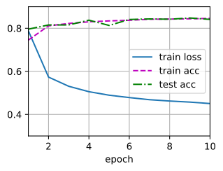
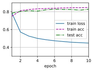
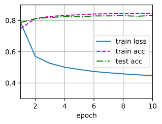
接下来我们调用 3.6节中 定义的训练函数来训练模型。

mxnetpytorchtensorflowpaddle

num_epochs = 10
d2l.train_ch3(net, train_iter, test_iter, loss, num_epochs, trainer)

num_epochs = 10
d2l.train_ch3(net, train_iter, test_iter, loss, num_epochs, trainer)

num_epochs = 10
d2l.train_ch3(net, train_iter, test_iter, loss, num_epochs, trainer)

num_epochs = 10
d2l.train_ch3(net, train_iter, test_iter, loss, num_epochs, trainer)

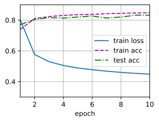
和以前一样，这个算法使结果收敛到一个相当高的精度，而且这次的代码比之前更精简了。

3.7.5. 小结

• 使用深度学习框架的高级API，我们可以更简洁地实现softmax回归。

• 从计算的角度来看，实现softmax回归比较复杂。在许多情况下，深度学习框架在这些著名的技巧之外采取了额外的预防措施，来确保数值的稳定性。这使我们避免了在实践中从零开始编写模型时可能遇到的陷阱。

3.7.6. 练习

1. 尝试调整超参数，例如批量大小、迭代周期数和学习率，并查看结果。

2. 增加迭代周期的数量。为什么测试精度会在一段时间后降低？我们怎么解决这个问题？

mxnetpytorchtensorflowpaddle

Discussions

Discussions

Discussions

Discussions