Diagonalization of a Matrix

The process of converting a square matrix into diagonal form using a similarity transformation is called diagonalization. A matrix A is diagonalizable if there exists an invertible matrix P and a diagonal matrix D such that:

Where:

• D contains the eigenvalues of A along its diagonal.
• P is the change of basis matrix, whose columns are the corresponding eigenvectors of A.

Diagonalization is useful because diagonal matrices are much easier to work with. For instance, raising a diagonal matrix to a power simply means raising its diagonal entries to that power, and its determinant is just the product of the diagonal entries.

Conditions

• A matrix is diagonalizable if and only if each eigenvalue’s geometric multiplicity (number of linearly independent eigenvectors) equals its algebraic multiplicity (its multiplicity as a root of the characteristic polynomial).
• An n×n matrix over a field F is diagonalizable if it has n linearly independent eigenvectors in F. This is always true if it has n distinct eigenvalues.

Change of Basis

Suppose we have a vector space V of dimension n over a field F.

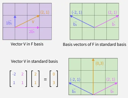
How do we convert the coordinates of v in basis F into coordinates in the standard basis.

• The change-of-basis matrix P contains the basis vectors of F expressed in terms of the standard basis.

When we multiply a vector v with the change-of-basis matrix, which is the matrix having basis vectors as columns, we get the coordinates of vector v in the standard basis.

Example: A vector in F-basis is converted to standard basis using the change-of-basis matrix.

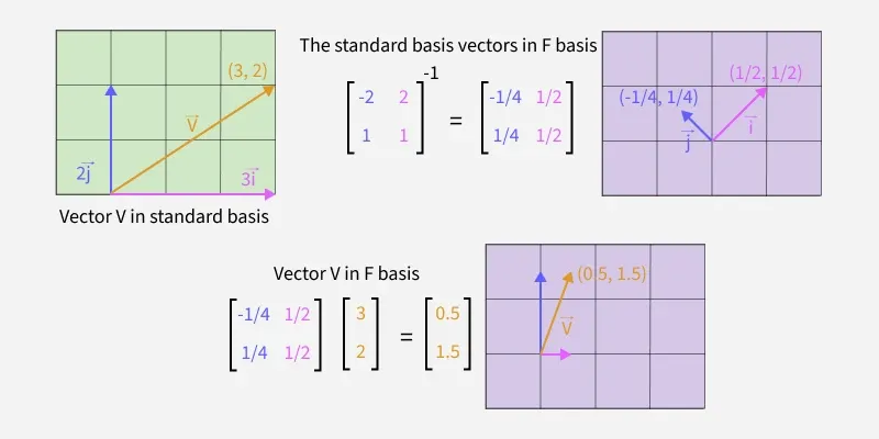
How do we convert the coordinates of v in the standard basis into coordinates in basis F.

• When we multiply a vector v with the inverse of the change-of-basis matrix, we get the coordinates of vector v in the F basis.

Example: A vector in F-basis is converted to standard basis using the change-of-basis matrix.

Procedure

The process of diagonalization can be visualized as switching into the eigenbasis, applying a simple scaling transformation, and then switching back to the standard basis. The following steps illustrate this process:

We write a matrix as:

A = PDP⁻¹

Where:

• P (Change-of-Basis Matrix): This matrix transforms coordinates into the new eigenvector system. Its columns are the eigenvectors of A.
• P⁻¹ (Inverse of P): This matrix transforms coordinates back from the eigenvector system to the standard system.
• D (Diagonal Matrix): This is the simple, "core" transformation in the new coordinate system. Its diagonal entries are the eigenvalues of A.

Steps:

• Find the eigenvalues (λ): Solve det(A - λI) = 0.
• Find the eigenvectors (v): For each eigenvalue λ, solve (A - λI) v = 0.
• Check for diagonalizability: Ensure you found n linearly independent eigenvectors. (If an eigenvalue with multiplicity m has fewer than m independent eigenvectors, A is not diagonalizable.)
• Construct matrix P that has the n eigenvectors as its columns.
• Construct matrix D is a diagonal matrix with the corresponding eigenvalues on the diagonal.
• Find P⁻¹.
• Write the factorization: A = PDP⁻¹

Diagonalizing a 2 × 2 matrix

A = \begin{bmatrix} 4 & 1\\ 2 & 3 \end{bmatrix}

A = PDP⁻¹

1. Find the eigenvalues:

det(A−λI) = 0

A−λI = \begin{bmatrix} 4 - \lambda & 1\\ 2 & 3 - \lambda \end{bmatrix}

det(A−λI) = (4 − λ)(3 − λ) - (1)(2) = λ² − 7λ + 12 − 2 = λ² − 7λ + 10

λ² − 7λ + 10 = 0 ⇒ (λ − 2)(λ − 5) = 0

Eigenvalues: λ₁ = 2, λ₂ = 5

2. Find the eigenvectors:

For λ₁ = 2,
Solve (A−2I)v = 0

A - 2I = \begin{bmatrix} 2 & 1\\ 2 & 1 \end{bmatrix}

2x + y = 0
2x + y = 0

v = \begin{bmatrix} x\\ -2x \end{bmatrix} = x \begin{bmatrix} 1\\ -2 \end{bmatrix}

v₁ = \begin{bmatrix} 1\\ -2 \end{bmatrix}

For λ2 = 5,
Solve (A − 5I)v = 0

A - 5I = \begin{bmatrix} -1 & 1\\ 2 & -2 \end{bmatrix}

-x + y = 0
2x - 2y = 0

x = y

v = \begin{bmatrix} x\\ x \end{bmatrix} = x \begin{bmatrix} 1\\ 1 \end{bmatrix}

v₂ = \begin{bmatrix} 1\\ 1 \end{bmatrix}

3. Constructing P and D:

P matrix: \begin{bmatrix} 1 & 1 \\ -2 & 1 \end{bmatrix}

D matrix: \begin{bmatrix} \lambda_1 & 0 \\ 0 & \lambda_2 \end{bmatrix} = \begin{bmatrix} 2 & 0 \\ 0 & 5 \end{bmatrix}

4. Finding P^-1_:

P = \begin{bmatrix} 1 & 1 \\ -2 & 1 \end{bmatrix} ⇒ P^-1 = \begin{bmatrix} \frac{1}{3} & -\frac{1}{3} \\ \frac{2}{3} & \frac{1}{3} \end{bmatrix}

5. Combining the terms:

PDP^-1 = \begin{bmatrix} 1 & 1 \\ -2 & 1 \end{bmatrix} \begin{bmatrix} \lambda_1 & 0 \\ 0 & \lambda_2 \end{bmatrix} = \begin{bmatrix} 2 & 0 \\ 0 & 5 \end{bmatrix} \begin{bmatrix} \frac{1}{3} & -\frac{1}{3} \\ \frac{2}{3} & \frac{1}{3} \end{bmatrix} = \begin{bmatrix} 4 & 1\\ 2 & 3 \end{bmatrix}

Diagonalizing a 3 × 3 matrix

A = \begin{bmatrix} -1 & 0 & 1\\3 & 0 & -3 \\ 1 & 0 & -1 \end{bmatrix}

A = PDP⁻¹

1. Find the eigenvalues:

det(A−λI) = 0

A−λI = \begin{bmatrix} -1 - \lambda & 0 & 1\\ 3 & - \lambda & -3 \\ 1 & 0 & -1-\lambda \end{bmatrix}

det(A−λI) = (−λ)⋅(1)⋅[(−1−λ)(−1−λ)−(1)(1)] = −λ³ - 2λ²

−λ³ - 2λ² = 0 ⇒ λ² (λ + 2)= 0

Eigenvalues: λ₁ = -2, λ₂ = 0, λ₃ = 0 (Note: λ = 0is an eigenvalue with algebraic multiplicity 2)

2. Find the eigenvectors:

For λ₁ = -2,
Solve (A−(-2)I)v = 0

A + 2I = \begin{bmatrix} 1 & 0 & 1\\ 3 & 2 & -3 \\ 1 & 0 & 1 \end{bmatrix}

x+z = 0 ⇒ x = −z

y − 3z = 0 ⇒ y = 3z

v = \begin{bmatrix} -z\\ 3z \\ z\end{bmatrix} = z \begin{bmatrix} -1\\ 3 \\ 1\end{bmatrix}

v₁ = \begin{bmatrix} -1\\ 3 \\ 1 \end{bmatrix}

For λ₂ =  λ₃ = 0,
Solve (A − 0I)v = 0

A = \begin{bmatrix} -1 & 0 & 1\\3 & 0 & -3 \\ 1 & 0 & -1 \end{bmatrix}

x − z = 0 ⇒ x = z

v = \begin{bmatrix} z\\ y \\z \end{bmatrix} = y \begin{bmatrix} 0\\ 1 \\0\end{bmatrix} + z \begin{bmatrix} 1\\ 0 \\1\end{bmatrix}

v₂ = \begin{bmatrix} 0\\ 1 \\ 0 \end{bmatrix}

v₃ = \begin{bmatrix} 1\\ 0 \\ 1 \end{bmatrix}

3. Constructing P and D:

P matrix: \begin{bmatrix} -1 & 0 & 1 \\ 3 & 1 & 0 \\ 1 & 0 & 1\end{bmatrix}

D matrix: \begin{bmatrix} -2 & 0 & 0 \\ 0 & 0 & 0 \\ 0 & 0 & 0\end{bmatrix}

4. Finding P^-1_:

P = \begin{bmatrix} -1 & 0 & 1 \\ 3 & 1 & 0 \\ 1 & 0 & 1\end{bmatrix} ⇒ P^-1 = \begin{bmatrix} -\frac{1}{2} & 0 & \frac{1}{2} \\ \frac{3}{2} & 1 & -\frac{3}{2} \\ \frac{1}{2} & 0 & \frac{1}{2} \end{bmatrix}

5. Combining the terms:

PDP^-1 = \begin{bmatrix} -1 & 0 & 1 \\ 3 & 1 & 0 \\ 1 & 0 & 1\end{bmatrix} \begin{bmatrix} -2 & 0 & 0 \\ 0 & 0 & 0 \\ 0 & 0 & 0\end{bmatrix} \begin{bmatrix} -\frac{1}{2} & 0 & \frac{1}{2} \\ \frac{3}{2} & 1 & -\frac{3}{2} \\ \frac{1}{2} & 0 & \frac{1}{2} \end{bmatrix} = \begin{bmatrix} -1 & 0 & 1\\3 & 0 & -3 \\ 1 & 0 & -1 \end{bmatrix}

Practice Questions

Question 1:  Determine if the given matrix is diagonalizable. If it is, find matrices P, D, and P⁻¹ such that A = PDP⁻¹. A = \begin{bmatrix} 5 & -1\\ -1 & 5 \end{bmatrix}.

Question 2: Determine if the given matrix is diagonalizable. If it is, find matrices P, D, and P⁻¹ such that A = PDP⁻¹. A = \begin{bmatrix} 4 & 0\\ 0 & 4 \end{bmatrix}.

Question 3: Determine if the given matrix is diagonalizable. If it is, find matrices P, D, and P⁻¹ such that A = PDP⁻¹. A = \begin{bmatrix} 3 & 1\\ 0 & 3 \end{bmatrix}.

Question 4: Determine if the given matrix is diagonalizable. If it is, find matrices P, D, and P⁻¹ such that A = PDP⁻¹. A = \begin{bmatrix} 1 & 2 & 2\\ 2 & 1 & 2\\2 & 2 & 1 \end{bmatrix}.

Answers:

1. P = \begin{bmatrix} 1 & -1\\ 1 & 1 \end{bmatrix}. D = \begin{bmatrix} 4 & 0\\ 0 & 6 \end{bmatrix}, P ^-1 =\begin{bmatrix} 1/2 & 1/2\\ -1/2 & 1/2 \end{bmatrix}

2. P = \begin{bmatrix} 1 & 0\\ 0 & 1 \end{bmatrix}. D = \begin{bmatrix} 4 & 0\\ 0 & 4 \end{bmatrix}, P ^-1 =\begin{bmatrix} 1 & 0\\ 0 & 1\end{bmatrix}

3. The matrix is non-diagonalizable because there is only one linearly independent eigenvectors for 2 x 2 matrix.

4. P = \begin{bmatrix} 1 & 1 & 1\\ 1 & -1 & 0\\ 1 & 0 & -1 \end{bmatrix}. D = \begin{bmatrix} 5 & 0 & 0\\ 0 & -1 & 0 \\ 0 & 0 & -1 \end{bmatrix}, P ^-1 =\frac{1}{3}\begin{bmatrix} 1 & 2 & 1\\ 1 & -2 & 1 \\ 1 & 1 & -2\end{bmatrix}