

Maximum Flow Problem is a graph optimization problem where the goal is to find the maximum amount of flow that can be sent from a source vertex to a sink vertex in a network. The network is represented as a directed graph in which:
- Vertices represent junctions or points in the network.
- Edges represent paths through which flow can travel.
- Each edge has a capacity that specifies the maximum amount of flow it can carry.
Example:
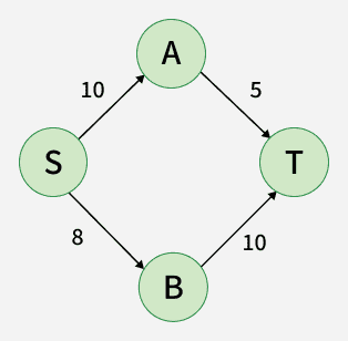
Imagine a water distribution system where water needs to be transported from a reservoir to a city through a network of pipes. Consider the following network:
Here:
- S is the source (reservoir).
- T is the sink (city).
- The number on each edge represents its capacity.
Step 1: Find Possible Paths. There are two paths from source to sink:
- S -> A -> T
- S -> B -> T
Step 2: Calculate Flow Through Each Path
- For the path: S -> A -> T. The capacities are: S -> A = 10 and A -> T = 5. Since a path can carry only as much flow as its smallest-capacity edge, this path can carry: min(10, 5) = 5 units of flow.
- For the second path: S -> B -> T. The capacities are: S -> B = 8 and B -> T = 10 This path can carry: min(8, 10) = 8 units of flow.
Step 3: Compute Total Flow
- The total flow reaching the sink is: 5 + 8 = 13 units.
- Thus, the maximum flow in this network is: 13 units.
Important Terminology
Consider the following network:
Source (S): The starting vertex from where the flow begins. Here, S is the source.
Sink (T): The destination vertex where the flow ends. Here, T is the sink.
Capacity: The maximum amount of flow an edge can carry. For example, the capacity of edge S -> A is 10.
Flow:
- Flow is the actual amount of flow sent through an edge.
- For example, if 5 units of flow are sent through edge S -> A, then the flow on that edge is 5.
- The flow on an edge cannot exceed its capacity.
Flow Conservation: For every intermediate vertex, incoming flow must equal outgoing flow. For example, if vertex A receives 5 units, it must also send 5 units.
Residual Capacity: It is the remaining capacity of an edge after some flow has been sent through it.
- It is calculated as: Residual Capacity = Capacity - Flow
- For example, if an edge has a capacity of 10 and currently carries 5 units of flow:
- Residual Capacity = 10 - 5 = 5, Therefore, 5 more units of flow can be sent through that edge in the forward direction.
Residual Graph: It is a graph that represents the remaining capacities of the edges in a flow network.
It helps identify where additional flow can be sent and allows previously sent flow to be adjusted during maximum-flow algorithms.
The residual graph may contain:
- Forward edges, representing the remaining capacity of the original edges.
- Reverse edges, representing the possibility of reducing previously sent flow.
Augmenting Path: A path from the source to the sink with positive residual capacity on every edge. For example, S -> A -> T is an augmenting path.
Bottleneck Capacity: The minimum capacity (or residual capacity) along an augmenting path. For S -> A -> T, the bottleneck is min(10, 5) = 5.
Maximum Flow: The largest amount of flow that can be sent from the source to the sink while satisfying all constraints. In the above network, the maximum flow is 5 + 8 = 13 units.
Applications of Maximum Flow
Maximum flow is used in various real-world and computational problems, such as:
- Network Routing: Maximizing data flow through communication networks.
- Transportation: Maximizing the movement of goods or vehicles through a road network.
- Water Distribution: Maximizing water flow through a system of pipes.
- Bipartite Matching: Finding the maximum number of possible matches.
- Job Assignment: Assigning jobs to workers subject to capacity constraints.
- Supply Chain: Maximizing the flow of products through a distribution network.
