Multivariate Time Series Forecasting with LSTMs in Keras

Multivariate time series forecasting is the task of predicting the future values of multiple related variables by learning from their past behaviour over time. Instead of modelling each variable separately, this approach captures how variables influence one another across time. When combined with Long Short-Term Memory (LSTM) networks, the model is able to learn both short-term variations and long-term trends.

Key Characteristics

• Multivariable Forecasting: The model predicts multiple time-dependent variables together, allowing it to capture how different features change and interact over time.
• Temporal Sequence Learning: Instead of using individual values, the model learns from sequences of past data, helping it understand trends and patterns across time.
• Long-Term Memory Capability: LSTM networks store important information from earlier time steps, making them effective for modelling long-term dependencies in time-series data.
• Inter-Feature Relationship Modeling: The model automatically learns how different variables influence each other, improving the accuracy of multivariate predictions.
• Efficient Modeling with Keras: Keras provides a simple and organised framework to build, train and evaluate LSTM-based forecasting models.

Step-by-Step Implementation

Let's see the implementation of Multivariate Time series Forecasting with LSTMs in Keras,

The used dataset can be downloaded from here.

Step 1: Import Libraries

We need to import the necessary libraries such as NumPy, Pandas, scikit learn, tensorflow, matplotlib and Keras.

import numpy as np
import pandas as pd
from sklearn.preprocessing import MinMaxScaler
from sklearn.metrics import mean_squared_error, mean_absolute_error, r2_score
import tensorflow as tf
from tensorflow import keras
import matplotlib.pyplot as plt

Step 2: Load Dataset

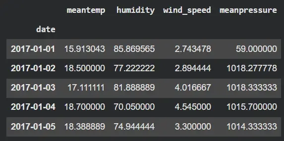
We will load the dataset:

• Reads the CSV file
• Converts the date column into datetime format
• Sets date as the index so the data has a real time order

You can download dataset from here.

df = pd.read_csv("/content/DailyDelhiClimateTest.csv")
df['date'] = pd.to_datetime(df['date'])
df.set_index('date', inplace=True)

df.head()

Output:

Step 3: Scale the Data

Here:

• Each climate variable is scaled between 0 and 1
• Prevents any one feature from dominating learning

scaler = MinMaxScaler()
scaled_data = scaler.fit_transform(df)

Step 4: Convert Time Series into Sequences

We transform the time-series data into sliding windows for LSTM input. This:

• Uses the last 20 days to predict the next day
• X contains sequences of past climate values
• y contains the future mean temperature

def create_sequences(data, window):
    X, y = [], []
    for i in range(len(data) - window):
        X.append(data[i:i + window])
        y.append(data[i + window, 0])
    return np.array(X), np.array(y)


X, y = create_sequences(scaled_data, 20)

Step 5: Split into Testing and Training Sets

We will split the dataset for training and testing sets:

split = int(0.85 * len(X))

X_train, X_test = X[:split], X[split:]
y_train, y_test = y[:split], y[split:]

Step 6: Built the LSTM Model

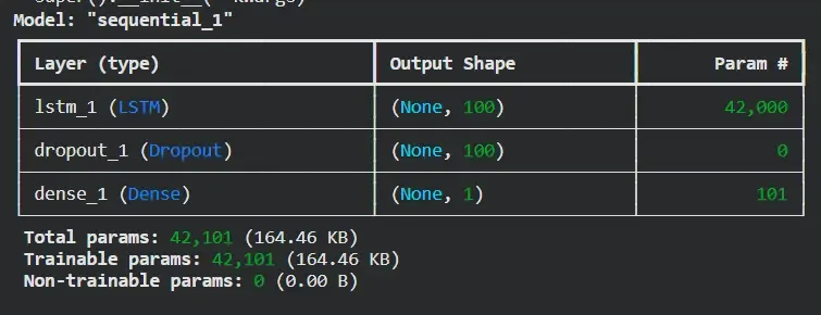
We will define the neural network structure. Here:

• LSTM learns time-based patterns
• Dropout reduces overfitting
• Dense layer outputs next-day temperature
• Mean squared error is used as loss

model = keras.Sequential()
model.add(keras.layers.LSTM(100, input_shape=(
    X_train.shape[1], X_train.shape[2])))
model.add(keras.layers.Dropout(0.2))
model.add(keras.layers.Dense(1))

model.compile(loss="mse", optimizer="adam", metrics=["mae"])
model.summary()

Output:

Step 7: Train the Model

The model learns weather patterns from historical data and the model trains for 30 epochs.

history = model.fit(X_train, y_train, epochs=30, batch_size=16)

Step 8: Generate Predictions

We will make predictions.

pred = model.predict(X_test)

Step 9: Convert Predictions to Real Values

Scaled values are converted back to real temperature values.

y_test_inv = scaler.inverse_transform(
    np.c_[y_test, np.zeros((len(y_test), df.shape[1] - 1))]
)[:, 0]

pred_inv = scaler.inverse_transform(
    np.c_[pred, np.zeros((len(pred), df.shape[1] - 1))]
)[:, 0]

Step 10: Plot Actual vs Predicted Values

We will plot the values.

time = df.index[-len(y_test):]

plt.figure(figsize=(10, 5))
plt.plot(time, y_test_inv, label="Actual")
plt.plot(time, pred_inv, linestyle="--", label="Predicted")

highlight = int(len(time) * 0.85)
plt.axvspan(time[highlight], time[-1], alpha=0.3)

plt.title("Delhi Climate LSTM Forecast")
plt.xlabel("Date")
plt.ylabel("Mean Temperature")
plt.legend()
plt.show()

Output:

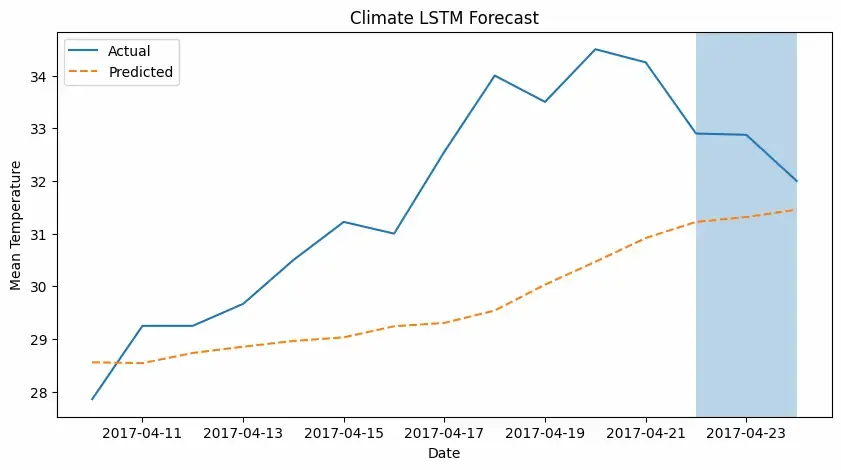
We can further improve our model by increasing number of epochs.

Step 11: Evaluate Model Performance

We evaluate the model performance,

• MSE shows squared error
• MAE shows average error
• R² shows how well predictions match actual values

mse = mean_squared_error(y_test_inv, pred_inv)
mae = mean_absolute_error(y_test_inv, pred_inv)
r2 = r2_score(y_test_inv, pred_inv)

mse, mae, r2

Output: