

Class imbalance occurs when certain classes in a dataset have far fewer samples compared to others. This imbalance can lead to models that are biased toward the majority class, reducing their ability to accurately predict the minority class. For example, in fraud detection, fraudulent transactions are rare compared to real ones. Without handling the imbalance, the model might simply predict all transactions as real, achieving high accuracy but failing to identify fraud. Addressing this issue is important for building models that generalize well across all classes.
Understanding class_weight in Keras
The class_weight parameter in Keras is a way to address class imbalance during model training. By assigning higher weights to underrepresented classes you make the model pay more attention to these classes. This helps to balance the learning process and ensure that the model does not become biased toward the majority class. The idea is to penalize the model more for making errors in minority classes, pushing it to learn better representations for them.
Scenarios Where Using class_weight Is Essential
Using class_weight is important in scenarios where class distributions are highly skewed. Some common examples include:
- Medical Diagnosis: Detecting rare diseases where the majority of patients are healthy.
- Fraud Detection: Identifying fraudulent transactions in a dataset dominated by legitimate transactions.
- Customer Churn Prediction: Predicting customer churn in a dataset where the majority of customers do not churn.
- Image Classification: Handling classes in image datasets that are significantly underrepresented.
Now we will discuss step by step implementation of How to Set class_weight in Keras Package using R Programming Language.
Step 1: Simulate an Imbalanced Dataset
First we will simulate an imbalanced dataset.
# Load necessary libraries
library(keras)
library(dplyr)

# Simulate dataset
set.seed(123)
x_train <- matrix(rnorm(1000 * 20), ncol = 20)
y_train <- c(rep(0, 900), rep(1, 100))  # Imbalanced: 900 of class 0, 100 of class 1

# Shuffle the data
shuffle_index <- sample(1:length(y_train))
x_train <- x_train[shuffle_index, ]
y_train <- y_train[shuffle_index]
Step 2: Analyze Class Distribution
Now we will Analyze Class Distribution.
# Check class distribution
class_distribution <- table(y_train)
print(class_distribution)
Output:
y_train
  0   1
900 100
Step 3: Calculate Class Weights
A common approach is to set the weights inversely proportional to the class frequencies. This means that classes with fewer samples get higher weights, and those with more samples get lower weights.
# Calculate class weights
total_samples <- sum(class_distribution)
num_classes <- length(class_distribution)
class_weights <- list(
    '0' = total_samples / (num_classes * class_distribution['0']),
    '1' = total_samples / (num_classes * class_distribution['1'])
)
print(class_weights)
Output:
$`0`
        0
0.5555556

$`1`
1
5
Step 4: Build a Simple Neural Network Model
Now we will Build a Simple Neural Network Model.
# Define model
model <- keras_model_sequential() %>%
  layer_dense(units = 32, activation = 'relu', input_shape = c(20)) %>%
  layer_dense(units = 1, activation = 'sigmoid')

model %>% compile(
  loss = 'binary_crossentropy',
  optimizer = optimizer_adam(),
  metrics = c('accuracy')
)
Step 5: Train the Model Without class_weight
Now we will Train the Model Without class_weight.
# Train without class_weight
history_no_weight <- model %>% fit(
  x_train, y_train,
  epochs = 10,
  batch_size = 32,
  validation_split = 0.2
)
Step 6: Train the Model With class_weight
Now we will Train the Model With class_weight.
# Train with class_weight
history_with_weight <- model %>% fit(
  x_train, y_train,
  epochs = 10,
  batch_size = 32,
  validation_split = 0.2,
  class_weight = class_weights
)
Step 7: Compare Results
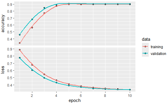
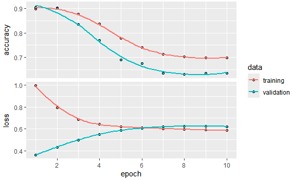
Now we will Compare Results by ploting both the plots.
# Plot training history for comparison
plot(history_no_weight)
plot(history_with_weight)

# Evaluate model without class_weight
eval_no_weight <- model %>% evaluate(x_train, y_train)
print("Performance metrics without class_weight:")
print(eval_no_weight)

# Evaluate model with class_weight
eval_with_weight <- model %>% evaluate(x_train, y_train)
print("Performance metrics with class_weight:")
print(eval_with_weight)

# Get predictions and compute precision and recall
predict_no_weight <- model %>% predict(x_train)
y_pred_no_weight <- ifelse(predict_no_weight > 0.5, 1, 0)

predict_with_weight <- model %>% predict(x_train)
y_pred_with_weight <- ifelse(predict_with_weight > 0.5, 1, 0)

# Load additional libraries for metrics
library(caret)

# Compute confusion matrices
confusion_no_weight <- confusionMatrix(factor(y_pred_no_weight), factor(y_train))
confusion_with_weight <- confusionMatrix(factor(y_pred_with_weight), factor(y_train))

print("Confusion Matrix without class_weight:")
print(confusion_no_weight)

print("Confusion Matrix with class_weight:")
print(confusion_with_weight)
Output:
Plotting model without class weight
Plotting model with class weight
[1] "Performance metrics without class_weight:"
$accuracy
[1] 0.712

$loss
[1] 0.5914723

[1] "Performance metrics with class_weight:"
$accuracy
[1] 0.712

$loss
[1] 0.5914723

[1] "Confusion Matrix without class_weight:"

 Confusion Matrix and Statistics

          Reference
Prediction   0   1
         0 646  34
         1 254  66

               Accuracy : 0.712
                 95% CI : (0.6828, 0.7399)
    No Information Rate : 0.9
    P-Value [Acc > NIR] : 1

                  Kappa : 0.191

 Mcnemar's Test P-Value : <2e-16

            Sensitivity : 0.7178
            Specificity : 0.6600
         Pos Pred Value : 0.9500
         Neg Pred Value : 0.2062
             Prevalence : 0.9000
         Detection Rate : 0.6460
   Detection Prevalence : 0.6800
      Balanced Accuracy : 0.6889

       'Positive' Class : 0

[1] "Confusion Matrix with class_weight:"

Confusion Matrix and Statistics

          Reference
Prediction   0   1
         0 646  34
         1 254  66

               Accuracy : 0.712
                 95% CI : (0.6828, 0.7399)
    No Information Rate : 0.9
    P-Value [Acc > NIR] : 1

                  Kappa : 0.191

 Mcnemar's Test P-Value : <2e-16

            Sensitivity : 0.7178
            Specificity : 0.6600
         Pos Pred Value : 0.9500
         Neg Pred Value : 0.2062
             Prevalence : 0.9000
         Detection Rate : 0.6460
   Detection Prevalence : 0.6800
      Balanced Accuracy : 0.6889

       'Positive' Class : 0
- Accuracy: Remains at 71.2% for both cases.
- Loss: Identical for both cases (0.5915).
- True Negatives (TN): 646
- False Positives (FP): 34
- True Positives (TP): 66
- False Negatives (FN): 254
- Sensitivity (Recall for class 0): 71.78%
- Specificity: 66.00%
- Precision (for class 0): 95.00%
- Balanced Accuracy: 68.89%
Conclusion
In Keras with R, setting and using class_weight involves defining a list of weights for each class, which adjusts the impact of each class on the model's training process. This can be achieved either by manual calculations based on the class frequencies or by using pre-defined weight adjustments. By combining class_weight into the fit function, you can ensure that the model learns effectively from all classes, helping to remove biases and improve overall performance.
