Uniform Cost Search (UCS) in AI

Uniform Cost Search (UCS) is an uninformed search algorithm that finds a least-cost path between a start node and a goal node in a weighted graph. Unlike methods that prioritize search depth, UCS evaluates paths according to the cost of reaching each node, making it useful for problems where different actions have different costs.

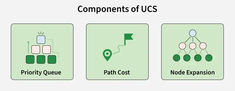
Key Concepts

• Priority Queue: Maintains the frontier of unexplored nodes and orders them by their current path cost, allowing UCS to consider the most promising low-cost node next.
• Path Cost and Optimality: Tracks the cumulative cost of reaching each node from the start. When edge costs are non-negative, selecting the goal from the lowest-cost position in the priority queue gives the minimum-cost solution.
• Node Expansion: Generates the successors of the selected node and adds or updates them in the frontier when a cheaper route to a successor is found.

Working

Uniform Cost Search (UCS) operates by always exploring the path with the lowest cumulative cost first. It uses a priority queue to keep track of nodes and their path costs.

1. Initialization: The algorithm begins at the starting node and assigns it a cost of 0 because no movement has been made yet.
2. Node Expansion: The node with the lowest path cost is selected from the priority queue and its neighboring nodes are explored.
3. Exploring Neighbors: For each neighboring node, UCS calculates the total cost to reach it from the start node. The node is then added to the priority queue or its cost is updated if a cheaper path is found.
4. Goal Check: After expanding a node, the algorithm checks if it has reached the goal node. If the goal is reached, the algorithm returns the total cost to reach this node and the path taken.
5. Repetition: This process repeats until the priority queue is empty or the goal is reached.

Implementation

Step 1: Import Required Libraries

Importing the required libraries for implementing Uniform Cost Search and visualizing the graph.

• heapq: Implements a priority queue for selecting the lowest-cost node.
• networkx: Used to create and manage graph structures.
• matplotlib.pyplot: Used to visualize the graph and highlight the shortest path.

import heapq
import networkx as nx
import matplotlib.pyplot as plt

Step 2: Define the Uniform Cost Search Function

This function implements the UCS algorithm to find the least cost path from a start node to a goal node in a weighted graph.

def uniform_cost_search(graph, start, goal):
    
    priority_queue = [(0, start)]
    # Dictionary to store the cost of the shortest path to each node
    visited = {start: (0, None)}
    
    while priority_queue:
        # Pop the node with the lowest cost from the priority queue
        current_cost, current_node = heapq.heappop(priority_queue)
        
        # If we reached the goal, return the total cost and the path
        if current_node == goal:
            return current_cost, reconstruct_path(visited, start, goal)
        
        # Explore the neighbors
        for neighbor, cost in graph[current_node]:
            total_cost = current_cost + cost
            # Check if this path to the neighbor is better than any previously found
            if neighbor not in visited or total_cost < visited[neighbor][0]:
                visited[neighbor] = (total_cost, current_node)
                heapq.heappush(priority_queue, (total_cost, neighbor))
    
    return None

Step 3: Define the Path Reconstruction Function

Creating a helper function to reconstruct the final path by tracing parent nodes from the goal back to the start.

def reconstruct_path(visited, start, goal):
    # Reconstruct the path from start to goal by following the visited nodes
    path = []
    current = goal
    while current is not None:
        path.append(current)
        current = visited[current][1]  # Get the parent node
    path.reverse()
    return path

Step 4: Define the Visualization Function

This function visualizes the graph and the path found by UCS, using networkx for graph creation and matplotlib for visualization.

def visualize_graph(graph, path=None):
    G = nx.DiGraph()

    # Adding nodes and edges to the graph
    for node, edges in graph.items():
        for neighbor, cost in edges:
            G.add_edge(node, neighbor, weight=cost)

    pos = nx.spring_layout(G)  # Positioning the nodes

    # Drawing the graph
    plt.figure(figsize=(8, 6))
    nx.draw(G, pos, with_labels=True, node_color='lightblue', node_size=2000, font_size=15, font_weight='bold', edge_color='gray')
    labels = nx.get_edge_attributes(G, 'weight')
    nx.draw_networkx_edge_labels(G, pos, edge_labels=labels, font_size=12)

    if path:
        # Highlight the path in red
        path_edges = list(zip(path, path[1:]))
        nx.draw_networkx_edges(G, pos, edgelist=path_edges, edge_color='red', width=2.5)

    plt.title("Uniform Cost Search Path Visualization")
    plt.show()

Step 5: Define the Graph and Execute UCS

Defining a sample graph as an adjacency list, set the start and goal nodes and run the UCS algorithm. It then visualizes the graph and the path found.

# Example graph represented as an adjacency list
graph = {
    'A': [('B', 1), ('C', 4)],
    'B': [('D', 1), ('E', 3)],
    'C': [('F', 5)],
    'D': [('G', 2)],
    'E': [('G', 1)],
    'F': [('G', 2)],
    'G': []
}

# Example usage of the UCS function
start_node = 'A'
goal_node = 'G'
result = uniform_cost_search(graph, start_node, goal_node)

if result:
    total_cost, path = result
    print(f"Least cost path from {start_node} to {goal_node}: {' -> '.join(path)} with total cost {total_cost}")
    visualize_graph(graph, path)
else:
    print(f"No path found from {start_node} to {goal_node}")

Output:

Least cost path from A to G: A -> B -> D -> G with total cost 4

You can download the complete code from here.

Applications

1. Pathfinding in Maps: Determining the shortest route between two locations on a map, considering different costs for different paths.
2. Network Routing: Finding the least-cost route in a communication or data network.
3. Puzzle Solving: Solving puzzles where each move has a cost associated with it, such as the sliding tiles puzzle.
4. Resource Allocation: Tasks that involve distributing resources efficiently, where costs are associated with different allocation strategies.

Advantages

• Optimality: Guarantees the optimal (minimum-cost) solution when all edge costs are non-negative.
• Completeness: Ensures a solution is found if a valid path to the goal exists.
• Cost-Based Exploration: Expands nodes based on cumulative path cost rather than depth, making it suitable for weighted graphs.
• Applicable to Variable Costs: Works effectively when actions or edges have different traversal costs.

Challenges

• High Time Complexity: May explore a large number of nodes before reaching the goal, especially in large search spaces.
• High Space Complexity: Requires storing all generated frontier nodes in the priority queue, leading to significant memory consumption.
• Repeated Node Expansions: Nodes may be revisited and updated when a lower-cost path is discovered.
• Performance Limitations: Can become computationally expensive for large graphs with many possible paths.