Greedy Best-First Search in AI

Greedy Best-First Search in AI is a heuristic search algorithm that selects the node that appears closest to the goal. It uses a heuristic function h(n) to estimate the remaining cost to the goal. Unlike A*, GBFS considers only the heuristic value and does not consider the cost already spent reaching a node.

Working

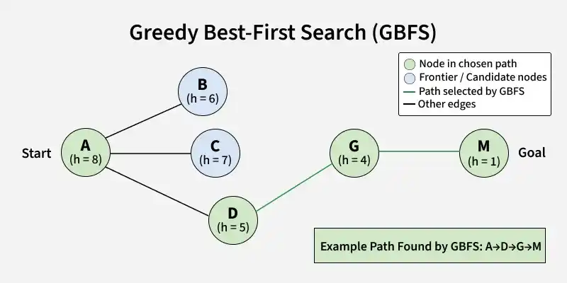
GBFS operates by exploring nodes in a graph by always choosing the one that appears closest to the goal. It’s called "greedy" because it selects the node that seems best at the moment based purely on this estimate, completely ignoring g(n) (the accumulated cost from the start node).

• Speed: Fast in practice because it prioritizes nodes that appear closest to the goal.
• Non-Optimal: Does not guarantee the shortest path because it ignores accumulated path costs (g(n)).
• Incomplete: Can get stuck in infinite loops in unbounded search spaces unless visited nodes are tracked.
• Backtracking Capability: Automatically switches to an alternative branch by pulling the next lowest heuristic node from its priority queue if a path leads to a dead end or high-cost nodes.

Step-by-Step Execution

1. Initialization: We start at the initial node and add it to a priority queue.
2. Expand Nodes: The algorithm evaluates all neighboring nodes, assigning each one a value based on the heuristic function (representing the estimated distance to the goal).
3. Select the Best Node: From the priority queue, the node with the lowest heuristic value is selected. This node is considered the most promising.
4. Goal Check: If the selected node is the goal, the search terminates. If not, the algorithm continues exploring.
5. Repeat: Steps 2-4 are repeated until the goal is found or the search space is exhausted.

Role of Heuristics in GBFS

The heuristic determines which node GBFS explores next.

Common heuristic function include:

• Euclidean Distance: Straight-line distance between the current node and the goal, used in pathfinding problems.
• Manhattan Distance: The sum of absolute differences between the coordinates of two points, often applied in grid-based environments.

A good heuristic can significantly reduce the number of nodes explored. However, GBFS does not guarantee that the heuristic will lead to the shortest path.

Example: Greedy Best-First Search for Hierarchical Routing

Consider a routing graph divided into three regions:

• Region 1: A, B, C
• Region 2: D, E, H, I, J
• Region 3: F, G, K, L, M

The objective is to find a path from node A to node M.

The region labels describe the structure of the graph, while GBFS uses the heuristic values to decide which node to explore next.

Step 1: Importing the Required Libraries

import heapq
import networkx as nx
import matplotlib.pyplot as plt

• heapq manages the priority queue based on min-heap operations.
• networkx is used handle graph creation and edge management.
• matplotlib generates visual plots of the graph and search path.

Step 2: Defining the Node Class

class Node:
    def __init__(self, name, heuristic):
        self.name = name
        self.heuristic = heuristic

    def __lt__(self, other):
        return self.heuristic < other.heuristic
      

• Creates a custom Node class storing a location name and its estimated goal distance (heuristic).
• Implements the __lt__ method to allow direct comparison, enabling heapq to sort nodes automatically by lowest heuristic value.

Step 3: Implementing Greedy Best-First Search Algorithm

def greedy_best_first_search_hierarchical(graph, start, goal, heuristic, region_map):
    priority_queue = []
    heapq.heappush(priority_queue, Node(start, heuristic[start]))
    
    visited = set()
    path = {start: None}
    
    while priority_queue:
        current_node = heapq.heappop(priority_queue).name
        
        if current_node == goal:
            return reconstruct_path(path, start, goal)
        
        visited.add(current_node)
        
        current_region = region_map[current_node]
        for neighbor in graph[current_node]:
            if neighbor not in visited and region_map[neighbor] == current_region:
                heapq.heappush(priority_queue, Node(neighbor, heuristic[neighbor]))
                if neighbor not in path:
                    path[neighbor] = current_node

        for neighbor in graph[current_node]:
            if neighbor not in visited and region_map[neighbor] != current_region:
                heapq.heappush(priority_queue, Node(neighbor, heuristic[neighbor]))
                if neighbor not in path:
                    path[neighbor] = current_node

    return None

• Initializes the priority queue, visited set and path dictionary.
• Expands nodes based on the lowest heuristic value, prioritizing same-region neighbors before inter-region neighbors.

Step 4: Reconstructing the Path

def reconstruct_path(path, start, goal):
    current = goal
    result_path = []
    while current is not None:
        result_path.append(current)
        current = path[current]
    result_path.reverse()
    return result_path

Step 5: Visualizing the Graph and Path

def visualize_graph(graph, path, pos, region_map):
    G = nx.Graph()
    for node, neighbors in graph.items():
        for neighbor in neighbors:
            G.add_edge(node, neighbor)

    plt.figure(figsize=(10, 8))
    nx.draw(G, pos, with_labels=True, node_size=4000, node_color='skyblue', 
            font_size=15, font_weight='bold', edge_color='gray')

    if path:
        path_edges = list(zip(path, path[1:]))
        nx.draw_networkx_edges(G, pos, edgelist=path_edges, edge_color='green', width=3)
        nx.draw_networkx_nodes(G, pos, nodelist=path, node_color='lightgreen')

    for node, region in region_map.items():
        plt.text(pos[node][0], pos[node][1] - 0.2, f"Region {region}", fontsize=12, color='black')

    plt.title("Greedy Best-First Search for Hierarchical Routing", size=20)
    plt.show()

• Creates a NetworkX graph instance and populates it with all nodes and connections.
• Renders base graph layout using fixed 2D coordinates (pos).
• Highlights the traversed result_path with green nodes and thick green edges, while labeling each node with its region index.

Step 6: Defining the Graph and Heuristic Values

graph = {
    'A': ['B', 'C'],
    'B': ['D', 'E'],
    'C': ['F', 'G'],
    'D': ['H'],
    'E': ['I', 'J'],
    'F': ['K' , 'M' , 'E'],
    'G': ['L', 'M'],
    'H': [],
    'I': [],
    'J': [],
    'K': [],
    'L': [],
    'M': []
}

heuristic = {
    'A': 8,
    'B': 6,
    'C': 7,
    'D': 5,
    'E': 4,
    'F': 5,
    'G': 4,
    'H': 3,
    'I': 2,
    'J': 1,
    'K': 3,
    'L': 2,
    'M': 1
}

region_map = {
    'A': 1, 'B': 1, 'C': 1,
    'D': 2, 'E': 2,
    'F': 3, 'G': 3,
    'H': 2, 'I': 2, 'J': 2,
    'K': 3, 'L': 3, 'M': 3
}

• Configures the graph adjacency list, connecting start node 'A' down through intermediate branches to leaves like 'M'.
• Assigns heuristic values representing straight-line distance estimates to goal 'M' (where h('M')=1).
• Maps nodes into distinct numerical regions (region_map) to enforce hierarchical constraints.

Step 7: Execute the Search and Visualize the Result

• Defines node positions for visualization and runs GBFS from A to M.
• Prints and visualizes the resulting path.

pos = {
    'A': (0, 0),
    'B': (-1, 1),
    'C': (1, 1),
    'D': (-1.5, 2),
    'E': (-0.5, 2),
    'F': (0.5, 2),
    'G': (1.5, 2),
    'H': (-2, 3),
    'I': (-1, 3),
    'J': (0, 3),
    'K': (1, 3),
    'L': (2, 3),
    'M': (3, 3)
}

start_node = 'A'
goal_node = 'M'
result_path = greedy_best_first_search_hierarchical(graph, start_node, goal_node, heuristic, region_map)

print("Path from {} to {}: {}".format(start_node, goal_node, result_path))

visualize_graph(graph, result_path, pos, region_map)

Output:

Path from A to M: ['A', 'C', 'G', 'M']

You can download the source code from here.

Applications

1. Pathfinding: Finding routes in maps, grids and virtual environments.
2. Game AI: Guiding characters or agents toward targets.
3. Robotics: Supporting heuristic-based navigation and path planning.
4. Puzzle Solving: Exploring promising states in problems such as sliding-tile puzzles.
5. Automated Planning: Searching large planning spaces where heuristic guidance can reduce exploration.

Advantages

1. Fast goal-directed search: The heuristic helps focus the search toward the goal.
2. Simple implementation: GBFS can be implemented using a heuristic and a priority queue.
3. Efficient exploration: A good heuristic can prevent the algorithm from exploring many irrelevant nodes.
4. Flexible: Different heuristics can be designed for different problem domains.
5. Useful for large search spaces: Heuristic guidance can make search practical when exhaustive exploration is expensive.

Limitations

1. Not optimal: GBFS does not guarantee the shortest or least-cost path.
2. Heuristic-sensitive: A poor heuristic can lead the search toward unproductive paths, while its effectiveness depends heavily on heuristic quality.
3. Memory Usage: GBFS can require substantial memory for its priority queue and visited nodes, with a worst-case space complexity of O(b^m). It may use less memory than A* when a strong heuristic keeps the search focused.
4. Ignores Path Cost: GBFS considers only the estimated distance to the goal, so tie-breaking between nodes with equal heuristic values can affect search behavior.