LLE: Locally Linear Embedding - A Nifty Way to Reduce Dimensionality in Python

Tips and Tricks, Machine Learning

Intro

It may be challenging to choose the right dimensionality reduction technique for your data. However, if you are specifically looking for a non-linear approach, then Locally Linear Embedding (LLE) and Isometric Mapping (Isomap) would be good ones to explore.

In this article, I will take you through the details of how LLE works and how it differs from Isomap. Also, I will provide a Python example to comparing these algorithms.

Contents

• LLE within the universe of Machine Learning algorithms

• Intuitive explanation of how LLE works

• Python example of LLE and its comparison to Isomap

Locally Linear Embedding (LLE) within the universe of Machine Learning algorithms

Even an experienced Data Scientist can easily get lost amongst hundreds of different Machine Learning algorithms used in the industry. Hence, I believe there is value in creating a structure by putting some of the most frequently used algorithms into categories.

It will never be perfect because some algorithms are flexible enough to perform multiple tasks. Nevertheless, below is my attempt to create such categorization. Make sure to explore this interactive graph by clicking👇 on different sections to reveal more.

As you can see, Locally Linear Embedding (LLE) sits under the Unsupervised branch of Machine Learning within the group of dimensionality reduction algorithms.

It means that you do not need to have a target variable to perform dimensionality reduction with LLE, unlike supervised techniques such as Linear Discriminant Analysis (LDA).

If you enjoy Data Science and Machine Learning, please subscribe to get an email whenever I publish a new story.

How does Locally Linear Embedding work?

The high-level steps

Similar to Isomap, LLE combines several steps to produce the lower-dimensional embedding. These are:

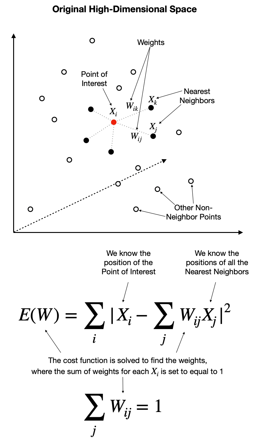
1. Use a KNN approach to find the k nearest neighbors of every data point. Here, "k" is an arbitrary number of neighbors that you can specify within model hyperparameters.

2. Construct a weight matrix where every point has its weights determined by minimizing the error of the cost function shown below. Note that every point is a linear combination of its neighbors, which means that weights for non-neighbors are 0.

1. Find the positions of all the points in the new lower-dimensional embedding by minimizing the cost function shown below. Note, here we use weights (W) from step two and solve for Y. The actual solving is performed using Partial Eigenvalue Decomposition.

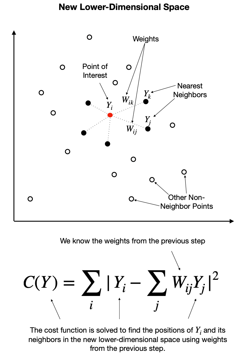
With the above steps completed, we get a lower-dimensional representation of the data, which we can typically visualize using standard scatterplots, provided we reduce the dimensionality to 3D or less.

LLE variants

You should be aware of a few LLE variants, which improve upon the original setup. However, note that these improvements come at the cost of efficiency, making the algorithm slower. Here is how scikit-learn describes these variants:

• Modified LLE (MLLE) - One well-known issue with LLE is the regularization problem. A way to address it is to use multiple weight vectors in each neighborhood. This is the essence of MLLE.

• Hessian LLE (HLLE)— Hessian Eigenmapping is another method of solving the regularization problem of LLE. It revolves around a hessian-based quadratic form at each neighborhood used to recover the locally linear structure.

While I will not go into details, I recommend you experiment with them to see which variant yields the best results for your data. Personally, I find MLLE to perform well in most scenarios (see an example of this in the next section).

Difference between LLE and Isomap

The two algorithms are similar in the way they approach dimensionality reduction, but they do have their differences.

Similar to LLE, Isomap also uses KNN to find the nearest neighbors in the first step. However, the second step constructs neighborhood graphs instead of describing each point as a linear combination of its neighbors. Then it uses these graphs to compute the shortest path between every pair of points.

Finally, Isomap uses those pairwise distances between all points to construct a lower-dimensional embedding.

Should I choose LLE over Isomap?

In general, LLE is a more efficient algorithm as it eliminates the need to estimate pairwise distances between widely separated data points. Furthermore, it assumes that the manifold is linear when viewed locally. Thus it recovers the non-linear structure from locally linear fits.

However, because LLE focuses on preserving only the local structures, it may introduce some unexpected distortions on the global scale.

In the Python section below, I use LLE, MLLE, and Isomap to create 2D embeddings of the 3D shape known as a "swiss roll." These examples should give you a good indication of the differences in results between these algorithms.

Python example of LLE and its comparison to Isomap

Setup

We will use the following data and libraries:

• Scikit-learn library for 1) creating the data (make_swiss_roll); 2) performing LLE and Modified LLE embeddings (LLE) 3) performing Isometric Mapping (Isomap);

Let's start by importing libraries.

# Data manipulationimport pandas as pd # for data manipulationimport numpy as np # for data manipulation# Visualizationimport plotly.express as px # for data visualization# Skleranfrom sklearn.datasets import make_swiss_roll # for creating swiss rollfrom sklearn.manifold import LocallyLinearEmbedding as LLE # for LLE dimensionality reductionfrom sklearn.manifold import Isomap # for Isomap dimensionality reduction

Next, we create data arrays containing swiss rolls using Sklearn's make_swiss_roll.

# Create a swiss rollX, y = make_swiss_roll(n_samples=2000, noise=0.05)# Make it thinnerX[:, 1] *= .5# Create a flat addon to the top of the swiss rollX_x=np.zeros((300,1))X_y=np.random.uniform(low=0, high=10, size=(300,1))X_z=np.random.uniform(low=14, high=25, size=(300,1))X2=np.concatenate((X_x, X_y, X_z), axis=1)y2=X_z.reshape(300)# Concatenate swiss roll and flat rectangle arraysX_two=np.concatenate((X, X2))y_two=np.concatenate((y, y2))

You will note that we have created two swiss rolls instead of one. The first one is standard, while the second one contains an additional rectangular addon at the top.

To see what I mean by this, let's first define two functions that we will use throughout the project to visualize our 3D swiss rolls and the 2D embedding results.

# Create a 3D scatter plotdef Plot3D(X, y, plot_name):    fig = px.scatter_3d(None,                         x=X[:,0], y=X[:,1], z=X[:,2],                        color=y,                        height=800, width=800                       )    # Update chart looks    fig.update_layout(title_text=plot_name,                      showlegend=False,                      legend=dict(orientation="h", yanchor="top", y=0, xanchor="center", x=0.5),                      scene_camera=dict(up=dict(x=0, y=0, z=1),                                             center=dict(x=0, y=0, z=-0.1),                                            eye=dict(x=1.5, y=1.75, z=1)),                                            margin=dict(l=0, r=0, b=0, t=0),                      scene = dict(xaxis=dict(backgroundcolor='white',                                              color='black',                                              gridcolor='#f0f0f0',                                              title_font=dict(size=10),                                              tickfont=dict(size=10),                                             ),                                   yaxis=dict(backgroundcolor='white',                                              color='black',                                              gridcolor='#f0f0f0',                                              title_font=dict(size=10),                                              tickfont=dict(size=10),                                              ),                                   zaxis=dict(backgroundcolor='lightgrey',                                              color='black',                                               gridcolor='#f0f0f0',                                              title_font=dict(size=10),                                              tickfont=dict(size=10),                                             )))    # Update marker size    fig.update_traces(marker=dict(size=3,                                   line=dict(color='black', width=0.1)))    fig.update(layout_coloraxis_showscale=False)    return fig#----------------------------------------------      # Create a 2D scatter plotdef Plot2D(X, y, plot_name):    # Create a scatter plot    fig = px.scatter(None, x=X[:,0], y=X[:,1],                      labels={                         "x": "Dimension 1",                         "y": "Dimension 2",                     },                     opacity=1, color=y)    # Change chart background color    fig.update_layout(dict(plot_bgcolor = 'white'))    # Update axes lines    fig.update_xaxes(showgrid=True, gridwidth=1, gridcolor='lightgrey',                      zeroline=True, zerolinewidth=1, zerolinecolor='lightgrey',                      showline=True, linewidth=1, linecolor='black')    fig.update_yaxes(showgrid=True, gridwidth=1, gridcolor='lightgrey',                      zeroline=True, zerolinewidth=1, zerolinecolor='lightgrey',                      showline=True, linewidth=1, linecolor='black')    # Set figure title    fig.update_layout(title_text=plot_name)    # Update marker size    fig.update_traces(marker=dict(size=5,                                 line=dict(color='black', width=0.3)))    return fig

Using the above Plot3D function, we can visualize our two swiss rolls:

Regular one:Plot3D(X, y, "Regular Swiss Roll")

Modified one:Plot3D(X_two, y_two, "Modified Swiss Roll")

Performing Locally Linear Embedding (LLE, MLLE) and Isomap

With setup complete, we will now perform dimensionality reduction using LLE, Modified LLE, and Isomap embeddings.

First, let's define a couple of reusable functions.

# Function for performing LLE and MLLEdef run_lle(num_neighbors, dims, mthd, data):    # Specify LLE parameters    embed_lle = LLE(n_neighbors=num_neighbors, # default=5, number of neighbors to consider for each point.                    n_components=dims, # default=2, number of dimensions of the new space                     reg=0.001, # default=1e-3, regularization constant, multiplies the trace of the local covariance matrix of the distances.                    eigen_solver='auto', # {'auto', 'arpack', 'dense'}, default='auto', auto : algorithm will attempt to choose the best method for input data                    #tol=1e-06, # default=1e-6, Tolerance for 'arpack' method. Not used if eigen_solver=='dense'.                    #max_iter=100, # default=100, maximum number of iterations for the arpack solver. Not used if eigen_solver=='dense'.                    method=mthd, # {'standard', 'hessian', 'modified', 'ltsa'}, default='standard'                    #hessian_tol=0.0001, # default=1e-4, Tolerance for Hessian eigenmapping method. Only used if method == 'hessian'                    modified_tol=1e-12, # default=1e-12, Tolerance for modified LLE method. Only used if method == 'modified'                    neighbors_algorithm='auto', # {'auto', 'brute', 'kd_tree', 'ball_tree'}, default='auto', algorithm to use for nearest neighbors search, passed to neighbors.NearestNeighbors instance                    random_state=42, # default=None, Determines the random number generator when eigen_solver == 'arpack'. Pass an int for reproducible results across multiple function calls.                    n_jobs=-1 # default=None, The number of parallel jobs to run. -1 means using all processors.                   )    # Fit and transofrm the data    result = embed_lle.fit_transform(data)    # Return results    return result#----------------------------------------------   # Function for performing Isomapdef run_isomap(num_neighbors, dims, data):    # Specify Isomap parameters    embed_isomap = Isomap(n_neighbors=num_neighbors, n_components=dims, n_jobs=-1)    # Fit and transofrm the data    result = embed_isomap.fit_transform(data)    # Return results    return result

We can now call the above functions to perform dimensionality reduction.

Let's create five 2D embeddings using different data and algorithms. Note that in all cases, we set the number of neighbors to 30 while using default values for other hyperparameters. Our five embeddings will be:

• Standard LLE on a regular swiss roll

• Modified LLE on a regular swiss roll

• Isomap on a regular swiss roll

• Modified LLE on a modified swiss roll

• Isomap on a modified swiss roll

######### Regular swiss roll ########## Standard LLE on a regular swiss rollstd_lle_res=run_lle(num_neighbors=30, dims=2, mthd='standard', data=X)# Modified LLE on a regular swiss rollmlle_res=run_lle(num_neighbors=30, dims=2, mthd='modified', data=X)# Isomap on a regular swiss rollisomap_res=run_isomap(num_neighbors=30, dims=2, data=X)######### Modified swiss roll ########## Modified LLE on a modified swiss rollmod_mlle_res=run_lle(num_neighbors=30, dims=2, mthd='modified', data=X_two)# Isomap on a modified swiss rollmod_isomap_res=run_isomap(num_neighbors=30, dims=2, data=X_two)

Finally, we can plot the results on 2D scatter plots using the Plot2D function we have created earlier.

Let's do it first on a regular swiss roll.

Plot2D(std_lle_res, y, 'Regular Swiss Roll - LLE')Plot2D(mlle_res, y, 'Regular Swiss Roll - MLLE')Plot2D(isomap_res, y, 'Regular Swiss Roll - Isomap')

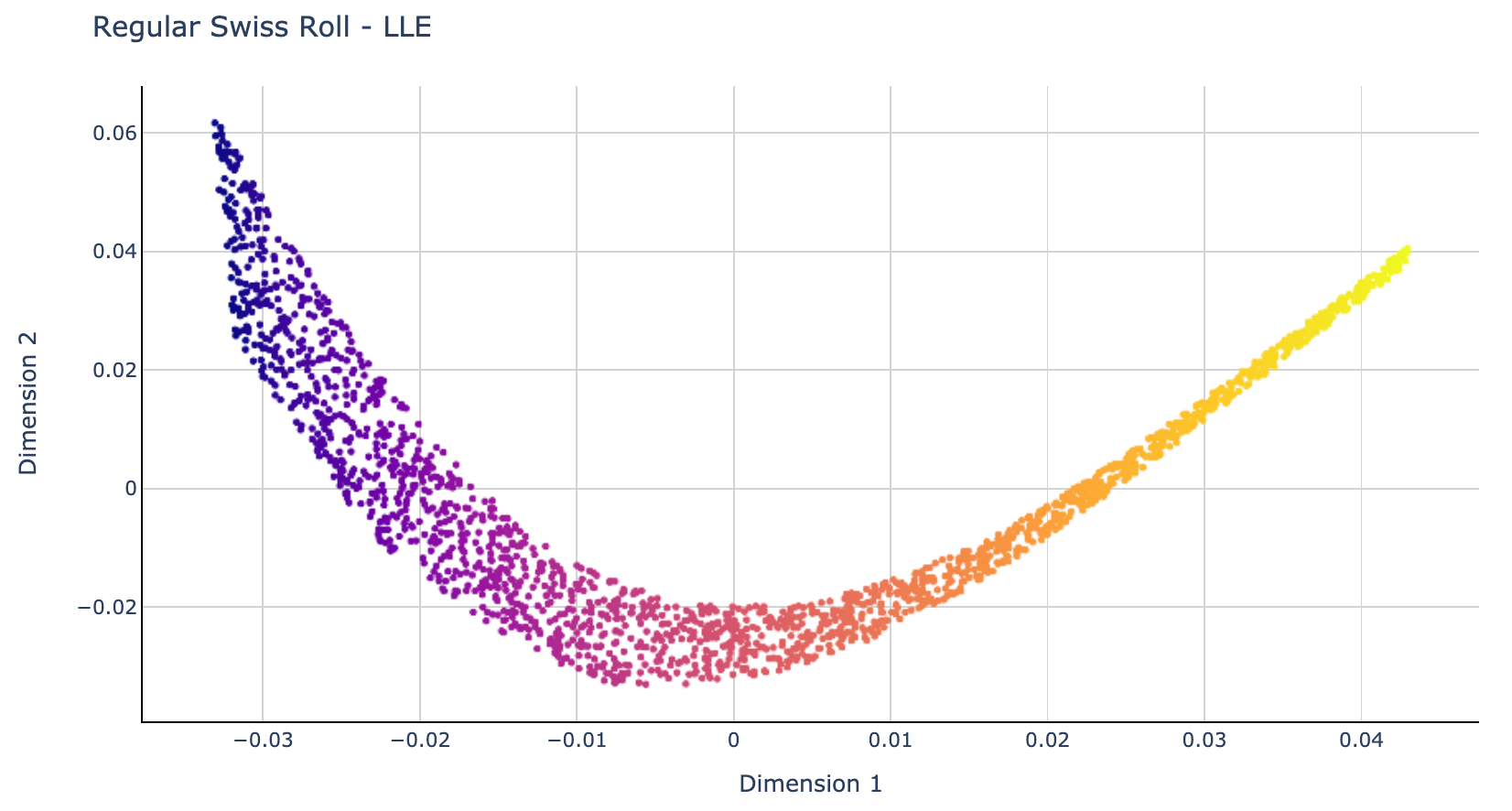
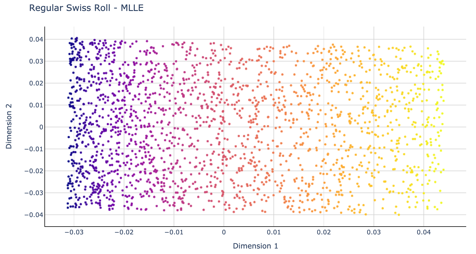
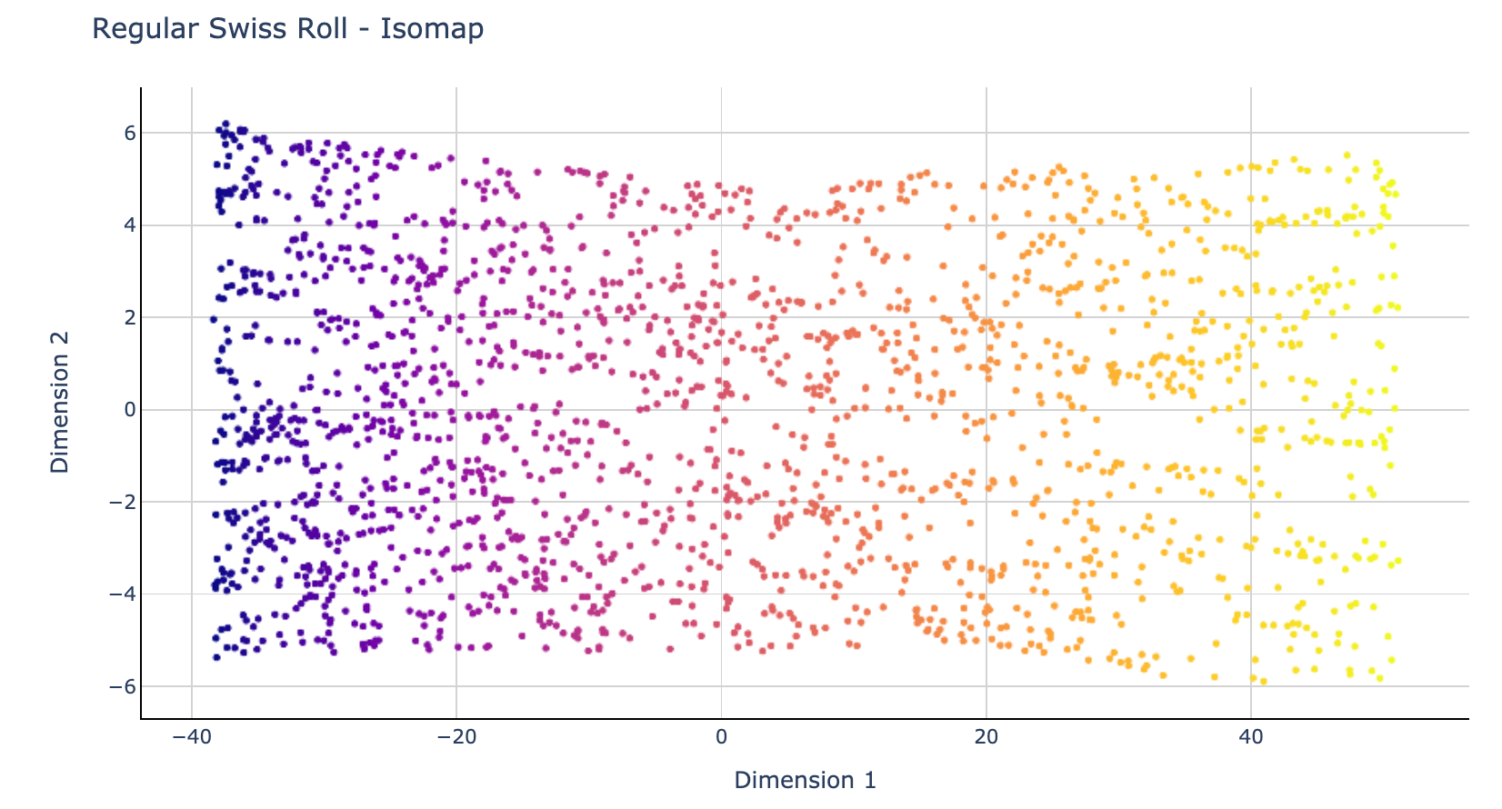
We can see that Standard LLE was not able to unroll the swiss roll successfully. By contrast, Modified LLE and Isomap did well, yielding similar results between them. In general, out of the three algorithms, MLLE seems to have the least distorted 2D embedding.

Next, let's visualize the results of the modified swiss roll embedding with MLLE and Isomap.

Plot2D(mod_mlle_res, y_two, 'Modified Swiss Roll - MLLE')Plot2D(mod_isomap_res, y_two, 'Modified Swiss Roll - Isomap')

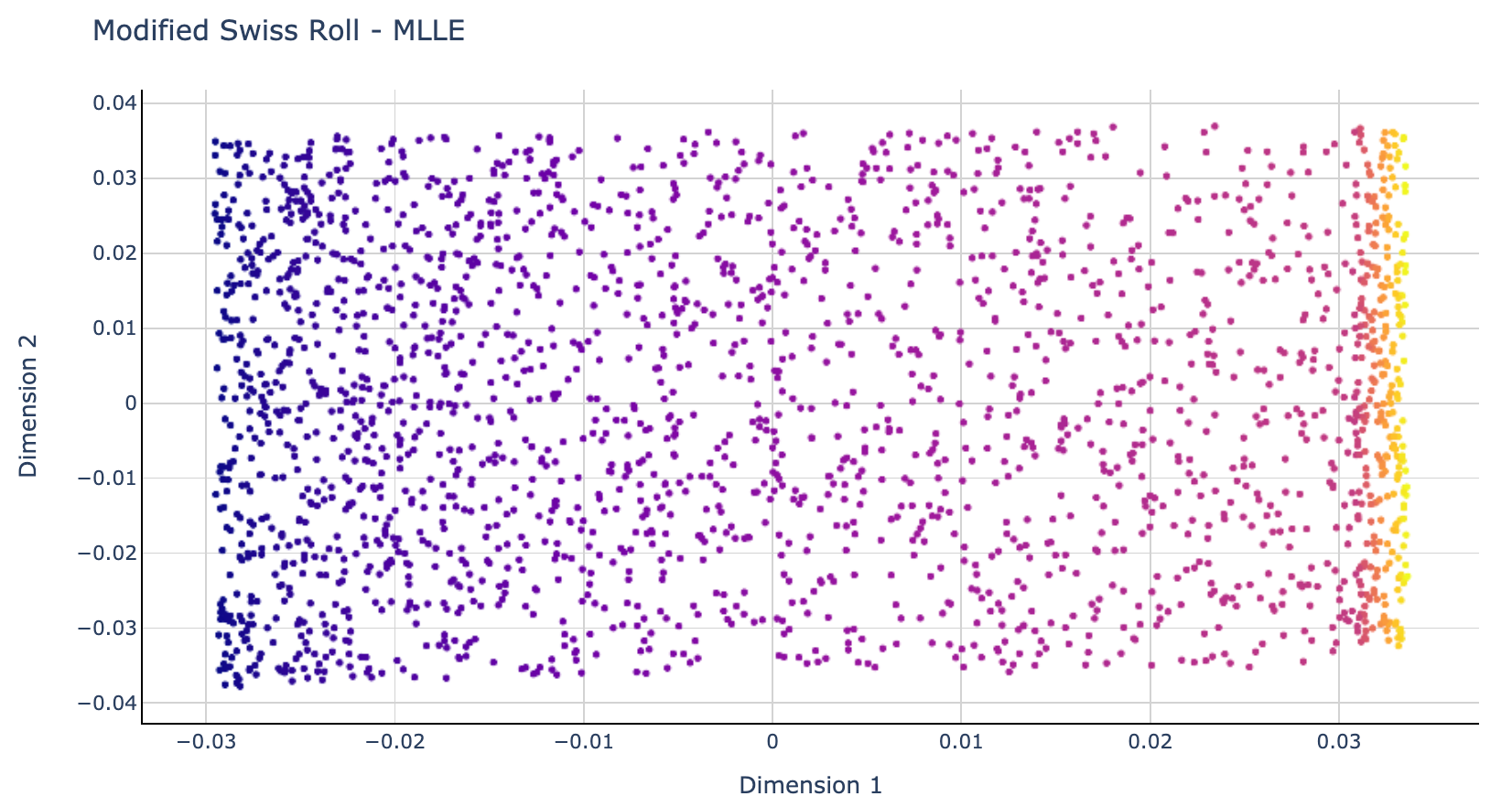
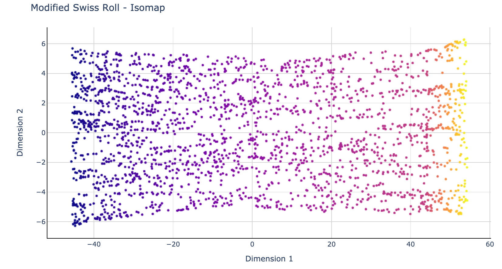
This time we can see more of a difference between the results of the two algorithms.

MLLE "struggled" to deal with different angles introduced to the 3D shape and ended up bunching all points from the rectangle part of the swiss roll closely together. Meanwhile, Isomap was able to flatten the whole structure pretty evenly.

Conclusions

Locally Linear Embedding (LLE) and especially the modified variant (MLLE) is an excellent tool to have within your arsenal.

With LLE being designed to focus on local structures, it can perform computations faster than other similar algorithms such as Isomap. However, choosing which algorithm you should use will depend on the data and the task you need to perform.

As with many cases in Data Science, you may want to experiment with a few different algorithms to find out which one does the best job for your data.

I sincerely hope you found my explanation and comparisons helpful. If you have any questions or suggestions, please do not hesitate to reach out.

Cheers 👏 Saul Dobilas

A couple of related articles you may find interesting:

Isomap Embedding - An Awesome Approach to Non-linear Dimensionality Reduction

t-SNE Machine Learning Algorithm - A Great Tool for Dimensionality Reduction in Python