




High-Performance Matrix Multiplication
This is a short post that explains how to write a high-performance matrix
multiplication program on modern processors. In this tutorial I will use a
single core of the Skylake-client CPU with AVX2, but the principles in this post
also apply to other processors with different instruction sets (such as AVX512).
Intro
Matrix multiplication is a mathematical operation that defines the product of
two matrices. It’s defined as
C(m, n) = A(m, k) * B(k, n)
It is implemented as a dot-product between the row matrix A and a column of
matrix B. In other words, it’s a sum over element-wise multiplication of two
scalars. And this is a naïve implementation in C:
for (int i = 0; i < m; i++) {
  for (int j = 0; j < n; j++) {
    for (int p = 0; p < k; p++) {
      C(i, j) += A(i, p) * B(p, j);
    }
  }
}
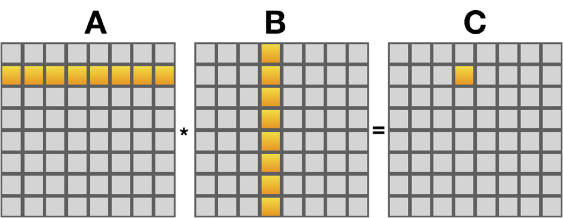
The picture below visualizes the computation of a single element in the result
matrix C. Each element in the result matrix C is the sum of element-wise
multiplication of a row from A and a column from B.
Performance analysis
The naïve implementation is pretty inefficient. In the next paragraph we’ll
estimate the capabilities of some processor in terms of flops/sec (floating
point operations per second). When you read the C code above try to guess how
efficient the naïve algorithm is. Can we make this program twice as fast? Maybe
more?
My laptop has an Intel Skylake processor with AVX2. This processor has two
execution ports that are capable of running 8-wide FMA (fused multiply-add)
instructions on each port every cycle. The machine runs at a frequency of about
4Ghz (let’s ignore Turbo in this discussion). To calculate the throughput of the
machine we’ll need to multiply these numbers together. 8 floating point numbers,
times two ports, times two (because we perform multiply and add together), times
4 giga hertz equals 128 Giga flops per second. (Giga is 1 followed by 9 zeros).
Now, let’s estimate how much work we need to perform. Let’s assume that we are
trying to multiply two matrices of size 1024 x 1024. The algorithm that we use
for matrix multiplication is O(n^3), and for each element we perform two
operations: multiplication and addition. The amount of compute that we need to
perform is 1024 ^ 3 * 2, which is about 2.1 Giga-flops. We should be able to
perform about 60 1024 x 1024 matrix multiplications per second if our code were
100% efficient and the program were not memory bound. This is the top of the
roof in the roofline model.
On my machine the naïve algorithm runs at around 8Gflops/sec. This is about 7%
utilization. In other words, the processor multipliers are idle 93% of the time.
Why is this program slow?
Our program is memory bound, which means that the multipliers are not active
most of the time because they are waiting for memory. One way to verify this
claim is to use performance counters. The two relevant counters are: the number
of executed AVX instructions, and the total number of cycle. When the code is
efficient, the number of AVX arithmetic operations is close to the total number
of cycles. If there’s a big gap between the two numbers, then we need to
investigate the cause. There are performance counters that record different
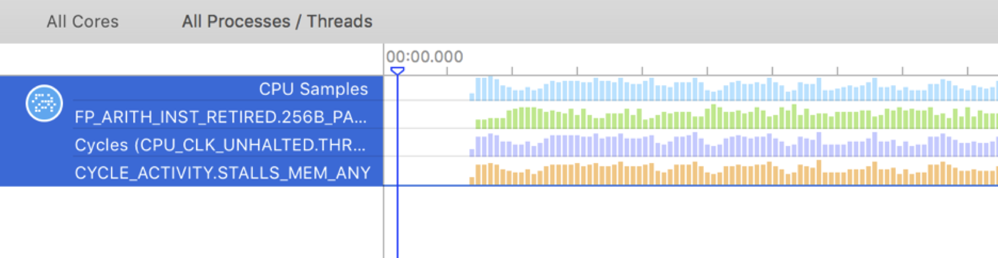
kinds of stalls, including memory stalls. This is a picture from Xcode’s
profiler that can record cpu performance counters.
Optimize the memory bandwidth
The CPU multipliers are not fully utilized because the naïve implementation
is memory bound. The processor is capable of loading wide SIMD vectors. On my
machine, using AVX, it’s 8 floating point numbers at once. In the case of matrix
A, the processor loads a cache line from the main memory into the L1 cache. Then it
loads the scalars from the cache line one at a time. This is not ideal, but the
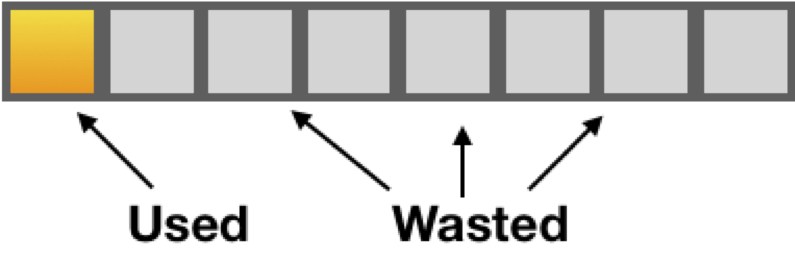
situation of matrix B is much much worse. In matrix B, we scan the matrix down a
column and use a single scalar from every cache line that we load. By the time
we finish scanning the column and start the next column, the processor had
already flushed the cache. Here I assume that the length of the column times
the size of the cache line is greater than our L1 cache. On my machine the L1
cache is 32K, and the size of the cache line is 64 bytes. This means that a
naïve scan of matrix with 512 rows would invalidate the L1 cache.
The first thing that we need to do to accelerate our program is to improve the
memory utilization of matrix B.
One possible implementation, which is kind of intuitive when you look at the
first diagram, is to use multiple scalar values from each cache line in matrix B
at once. We need to multiply the value that we load from matrix A with 8
consecutive values from matrix B. We can load a scalar from matrix A and
broadcast it 8 times to fill the SIMD register. Then, we can load 8 consecutive
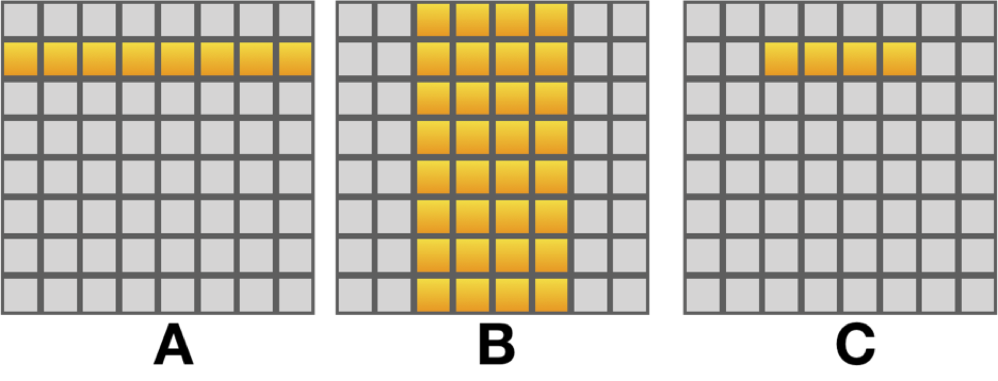
columns from matrix B and perform the vectorized element-wise computation. This
means that we process and calculate 8 results in matrix C at once. The picture
below depicts the vectorized matrix multiplication. Notice that instead of
accumulating into a single scalar we’ll be accumulating into a short vector of 8
scalars. The vectorized method will calculate 8 values in matrix C together.
This transformation reduces the memory bandwidth of matrix B by a factor of 8
(the SIMD width). Instead of performing N*N reads (that most likely miss the
cache) we perform N*N/8 reads.
Now that we’ve optimized the bandwidth of matrix B, let’s look at our CPU
architecture again. Our machine has two FMA ports, and two memory ports. This
means that we can load two elements from memory each cycle and perform two
arithmetic operations each cycle. However, in our algorithm we multiply an
element from matrix A with an element from matrix B. This means that we have two
memory operations for every arithmetic operation. Half of the time our
multipliers are waiting for data to be read from memory. In other words, our
current implementation can achieve at most 50% utilization.
Register Blocking
To get from 50% utilization to 100% utilization we need to perform one memory
operation for every arithmetic operation. The technique that people use is
called “register blocking”. It sounds scary, but it’s actually very simple.
After loading a value from memory, we need to use it more than once when
performing arithmetic calculations. Every value that we load from matrix A
should be multiplied with several values from matrix B, and every value that we
load from matrix B should be multiplied with several values from matrix A. Take
a look at the diagram below. Instead of calculating a single scalar in matrix C
we calculate a small patch. We accumulate into a number of registers at once.
The templated code below implements the innermost loops that calculate a patch
of size regA x regB in matrix C. The code loads regA scalars from matrixA
and regB SIMD-width vectors from matrix B. The program uses Clang’s extended
vector syntax.
/// Compute a RAxRB block of C using a vectorized dot product, where RA is the
/// number of registers to load from matrix A, and RB is the number of registers
/// to load from matrix B.
template <unsigned regsA, unsigned regsB>
void matmul_dot_inner(int k, const float *a, int lda, const float *b, int ldb,
                      float *c, int ldc) {
  float8 csum[regsA][regsB] = {{0.0}};
  for (int p = 0; p < k; p++) {

    // Perform the DOT product.
    for (int bi = 0; bi < regsB; bi++) {
      float8 bb = LoadFloat8(&B(p, bi * 8));
      for (int ai = 0; ai < regsA; ai++) {
        float8 aa = BroadcastFloat8(A(ai, p));
        csum[ai][bi] += aa * bb;
      }
    }
  }

  // Accumulate the results into C.
  for (int ai = 0; ai < regsA; ai++) {
    for (int bi = 0; bi < regsB; bi++) {
      AdduFloat8(&C(ai, bi * 8), csum[ai][bi]);
    }
  }
}
The C++ code above compiles to the assembly sequence below where RegA = 3, and
RegB = 4. You’ll notice that all of the arithmetic operations (vfmadd231ps)
operate directly on registers. This is a good thing because the values that are
loaded from matrix A and matrix B are reused by multiple arithmetic
instructions.
 nop
 vbroadcastss        (%rsi), %ymm12
 vmovups             -96(%rdx), %ymm13
 vfmadd231ps         %ymm13, %ymm12, %ymm11
 vbroadcastss        (%r13), %ymm14
 vfmadd231ps         %ymm13, %ymm14, %ymm9
 vbroadcastss        (%rbx), %ymm15
 vfmadd231ps         %ymm13, %ymm15, %ymm5
 vmovups             -64(%rdx), %ymm13
 vfmadd231ps         %ymm12, %ymm13, %ymm10
 vfmadd231ps         %ymm13, %ymm14, %ymm7
 vfmadd231ps         %ymm13, %ymm15, %ymm3
 vmovups             -32(%rdx), %ymm13
 vfmadd231ps         %ymm12, %ymm13, %ymm8
 vfmadd231ps         %ymm14, %ymm13, %ymm4
 vfmadd231ps         %ymm13, %ymm15, %ymm1
 vmovups             (%rdx), %ymm13
 vfmadd231ps         %ymm12, %ymm13, %ymm6
 vfmadd231ps         %ymm14, %ymm13, %ymm2
 vfmadd231ps         %ymm15, %ymm13, %ymm0
 addq                $4, %rbx
 addq                $4, %r13
 addq                $4, %rsi
 addq                %r11, %rdx
 addq                $-1, %r14
 jne                 "matmul-f+0x490"
Selecting the optimal register block parameters
How do we decide how many elements to load from matrix A and how many from
matrix B? One thing that we need to notice is that the number of registers is
limited. AVX2 can only encode 16 registers, which means that the size of the
patch in matrix C that we can calculate can be at most 16 * SIMD-width.
The configuration that we pick needs to minimize the ratio between the number of
memory operations and the number of arithmetic operations. The table below
lists a few possible register blocking values and their properties. The memory
operations column is calculated as RegA + RegB, because we need to load all of
the registers from memory. The arithmetic operations column is calculated as
RegA * RegB because we are multiplying each value from A with each value from
B. The total number of registers used is calculated as the number of
accumulation registers plus the number of registers from matrix A, that we
broadcast values into.
| Regs A | Regs B | Registers Used | Memory Ops | Arithmetic Ops |
|---|---|---|---|---|
| 1 | 4 | 5 | 5 | 4 |
| 2 | 4 | 10 | 6 | 8 |
| 2 | 5 | 12 | 7 | 10 |
| 4 | 3 | 16 | 7 | 12 |
| 1 | 8 | 9 | 9 | 8 |
| 3 | 4 | 15 | 7 | 12 |
As you can see in the table, when we select RegA = 3 and RegB = 4 we get the
best compute-to-memory ratio while still using less than 16 registers.
FMA utilization of register blocking
On Skylake the FMA execution ports are pipelined and have a latency of 5 cycles.
This means that to keep two FMA ports busy we need 10 independent chains of
computation. If we were to execute the code C += A * B in a loop then we would
need to wait 5 cycles before each iteration, because the current C would depend
on the result of the previous C, and the utilization of the machine would be
at most 20%.
When we block our registers with the parameters 3x4 we ensure that we have 12
independent chains of calculation that ensure that our FMA ports are always
busy. If we had decided to use register blocking of 2x4 then our FMAs would
only have 8 independent chains of calculation, which would result in only 80%
utilization because only 8 values would be processed at once, instead of 10.
The high-performance Convolution implementation in
Glow uses a 2x5 register blocking
implementation because these dimensions happen to work better for the shapes of
the matrices used.
Tiling
Register Blocking significantly reduces the number of times we load elements
from matrix B. However, our memory access pattern is still inefficient. We
access matrix B many times and multiply the values with different parts of
matrix A. As a result, we load matrix B into our cache, and then invalidate
this cache by loading a different part of matrix B.
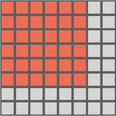
We now know how to calculate a patch in the output matrix C. Notice that the
order in which we calculate patches in matrix C affects the order in which we
access memory in matrix A and B. An ideal memory access pattern would be one
where we load matrix B into our L1 cache and keep it there for a long time. One
way to make this happen is to tile the calculation of matrix C. This is pretty
easy to do, just divide matrix C into small tiles (say, 128 x 256) and
calculate the results in C one patch at a time.
Conclusion
The register-blocked matrix multiplication is implemented in the
Glow compiler.
The code is very similar to the code in this post, except that it also handles
matrices with dimensions that are not a multiplication of the SIMD width. On my
machine the code runs at around 100 Gflops, which is not far from the
theoretical peak, and similar to Intel’s optimized implementation. To see what else can be done I recommend
reading this paper by Kazushige Goto.
The high-performance implementations of matrix multiplication is actually kind
of strange: load 3 scalars from the left-hand-side matrix and broadcast them
into full SIMD registers, then load 4 vector values from the right-hand-side
matrix, and multiply all of them into 12 accumulation registers. This odd
implementation is not something that the compiler can do for you
automatically.


 扫一扫
扫一扫


 276
276

 被折叠的 条评论
为什么被折叠?
被折叠的 条评论
为什么被折叠?
 到【灌水乐园】发言


